![]()
In this chapter, we dive into the basic modeling capabilities of CP-SAT. CP-SAT
provides an extensive set of constraints, closer to high-level modeling
languages like MiniZinc than to traditional Mixed Integer Programming (MIP). For
example, it offers constraints like all_different and
add_multiplication_equality. These advanced features reduce the need for
modeling complex logic strictly through linear constraints, though they also
increase the interface's complexity. However, not all constraints are equally
efficient; linear and boolean constraints are generally most efficient, whereas
constraints like add_multiplication_equality can be significantly more
resource-intensive.
Tip
If you are transitioning from Mixed Integer Programming (MIP), you might be used to manually implementing higher-level constraints and optimizing Big-M parameters for better performance. With CP-SAT, such manual adjustments are generally unnecessary. CP-SAT operates differently from typical MIP solvers by relying less on linear relaxation and more on its underlying SAT-solver and propagators to efficiently manage logical constraints. Embrace the higher-level constraints—they are often more efficient in CP-SAT.
This primer has been expanded to cover all constraints across two chapters, complete with various examples to illustrate the contexts in which they can be used. However, mastering modeling involves much more than just an understanding of constraints. It requires a deep appreciation of the principles and techniques that make models effective and applicable to real-world problems.
For a more detailed exploration of modeling, consider "Model Building in Mathematical Programming" by H. Paul Williams, which offers extensive insight into the subject, including practical applications. While this book is not specific to CP-SAT, the foundational techniques and concepts are broadly applicable. Additionally, for those new to this area or transitioning from MIP solutions, studying Gurobi's modeling approach through this video course might prove helpful. While many principles overlap, some strategies unique to CP-SAT can better address cases where traditional MIP-solvers struggle.
Additional resources on mathematical modeling (not CP-SAT specific):
- Math Programming Modeling Basics by Gurobi: This resource provides a solid introduction to the basics of mathematical modeling.
- Modeling with Gurobi Python: A comprehensive video course on modeling with Gurobi, highlighting concepts that are also applicable to CP-SAT.
- Model Building in Mathematical Programming by H. Paul Williams: An extensive guide to mathematical modeling techniques.
Elements:
- Variables:
new_int_var,new_bool_var,new_constant,new_int_var_series,new_bool_var_series- Custom Domain Variables:
new_int_var_from_domain
- Custom Domain Variables:
- Objectives:
minimize,maximize - Linear Constraints:
add,add_linear_constraint - Logical Constraints (Propositional Logic):
add_implication,add_bool_or,add_at_least_one,add_at_most_one,add_exactly_one,add_bool_and,add_bool_xor - Conditional Constraints (Reification):
only_enforce_if - Absolute Values and Max/Min:
add_min_equality,add_max_equality,add_abs_equality - Multiplication, Division, and Modulo:
add_modulo_equality,add_multiplication_equality,add_division_equality - All Different:
add_all_different - Domains and Combinations:
add_allowed_assignments,add_forbidden_assignments - Array/Element Constraints:
add_element,add_inverse
The more advanced constraints add_circuit, add_multiple_circuit,
add_automaton,add_reservoir_constraint,
add_reservoir_constraint_with_active, new_interval_var,
new_interval_var_series, new_fixed_size_interval_var,
new_optional_interval_var, new_optional_interval_var_series,
new_optional_fixed_size_interval_var,
new_optional_fixed_size_interval_var_series, add_no_overlap,
add_no_overlap_2d, and add_cumulative are discussed in the next chapter.
There are two important types of variables in CP-SAT: Booleans and Integers (which are actually converted to Booleans, but more on this later). There are also, e.g., interval variables, but they are actually rather a combination of integral variables and discussed later. For the integer variables, you have to specify a lower and an upper bound.
model = cp_model.CpModel()

# Integer variable z with bounds -100 <= z <= 100
z = model.new_int_var(-100, 100, "z")  # new syntax
z_ = model.NewIntVar(-100, 100, "z_")  # old syntax

# Boolean variable b
b = model.new_bool_var("b")  # new syntax
b_ = model.NewBoolVar("b_")  # old syntax

# Implicitly available negation of b:
not_b = ~b  # will be 1 if b is 0 and 0 if b is 1
not_b_ = b.Not()  # old syntax
Additionally, you can use model.new_int_var_series and
model.new_bool_var_series to create multiple variables at once from a pandas
Index. This is especially useful if your data is given in a pandas DataFrame.
However, there is no performance benefit in using this method, it is just more
convenient.
model = cp_model.CpModel()

# Create an Index from 0 to 9
index = pd.Index(range(10), name="index")

# Create a pandas Series with 10 integer variables matching the index
xs = model.new_int_var_series("x", index, 0, 100)

# List of boolean variables
df = pd.DataFrame(
    data={"weight": [1 for _ in range(10)], "value": [3 for _ in range(10)]},
    index=["A", "B", "C", "D", "E", "F", "G", "H", "I", "J"],
)
bs = model.new_bool_var_series("b", df.index)  # noqa: F841

# Using the dot product on the pandas DataFrame is actually a pretty
# convenient way to create common linear expressions.
model.add(bs @ df["weight"] <= 100)
model.maximize(bs @ df["value"])
Additionally, there is the new_constant-method, which allows you to create a
variable that is constant. This allows you to safely replace variables by
constants. This is primarily useful for boolean variables, as constant integer
variables can in most cases be simply replaced by plain integers.
Tip
In an older project, I observed that maintaining tight bounds on integer variables can significantly impact performance. Employing a heuristic to find a reasonable initial solution, which then allowed for tighter bounds, proved worthwhile, even though the bounds were just a few percent tighter. Although this project was several years ago and CP-SAT has advanced considerably since then, I still recommend keeping the bounds on the variables' ranges as tight as possible.
There are no continuous/floating point variables (or even constants) in CP-SAT: If you need floating point numbers, you have to approximate them with integers by some resolution. For example, you could simply multiply all values by 100 for a step size of 0.01. A value of 2.35 would then be represented by 235. This could probably be implemented in CP-SAT directly, but doing it explicitly is not difficult, and it has numerical implications that you should be aware of.
The absence of continuous variables may appear as a substantial limitation, especially for those with a background in linear optimization where continuous variables are typically regarded as the simpler component. However, if your problem includes only a few continuous variables that must be approximated using large integers and involves complex constraints such as absolute values, while the majority of the problem is dominated by logical constraints, CP-SAT can often outperform mixed-integer programming solvers. It is only when a problem contains a substantial number of continuous variables and benefits significantly from strong linear relaxation that mixed-integer programming solvers will have a distinct advantage, despite CP-SAT having a propagator based on the dual simplex method.
I analyzed the impact of resolution (i.e., the factor by which floating point numbers are multiplied) on the runtime of CP-SAT, finding that the effect varied depending on the problem. For one problem, the runtime increased only logarithmically with the resolution, allowing the use of a very high resolution of 100,000x without significant issues. In contrast, for another problem, the runtime increased roughly linearly with the resolution, making high resolutions impractical. The runtime for different factors in this case was: 1x: 0.02s, 10x: 0.7s, 100x: 7.6s, 1000x: 75s, and 10,000x: over 15 minutes, even though the solution remained the same, merely scaled. Therefore, while high resolutions may be feasible for some problems using CP-SAT, it is essential to verify their influence on runtime, as the impact can be considerable.
In my experience, boolean variables are crucial in many combinatorial optimization problems. For instance, the famous Traveling Salesman Problem consists solely of boolean variables. Therefore, implementing a solver that specializes in boolean variables using a SAT-solver as a foundation, such as CP-SAT, is a sensible approach. CP-SAT leverages the strengths of SAT-solving techniques, which are highly effective for problems dominated by boolean variables.
You may wonder why it is necessary to explicitly name the variables in CP-SAT. While there does not appear to be a technical reason for this requirement, naming the variables can be extremely helpful for debugging purposes. Understanding the naming scheme of the variables allows you to more easily interpret the internal representation of the model, facilitating the identification and resolution of issues. To be fair, there have only been a few times when I actually needed to take a closer at the internal representation, and in most of the cases I would have preferred not to have to name the variables.
When dealing with integer variables that you know will only need to take certain
values, or when you wish to limit their possible values, custom domain variables
can become interesting. Unlike regular integer variables, which must have a
domain between a given range of values (e.g.,
CP-SAT works by converting all integer variables into boolean variables (warning: simplification). For each potential value, it creates two boolean variables: one indicating whether the integer variable is equal to this value, and another indicating whether it is less than or equal to it. This is called an order encoding. At first glance, this might suggest that using domain variables is always preferable, as it appears to reduce the number of boolean variables needed.
However, CP-SAT employs a lazy creation strategy for these boolean variables. This means it only generates them as needed, based on the solver's decision-making process. Therefore, an integer variable with a wide range - say, from 0 to 100 - will not immediately result in 200 boolean variables. It might lead to the creation of only a few, depending on the solver's requirements.
Limiting the domain of a variable can have drawbacks. Firstly, defining a domain explicitly can be computationally costly and increase the model size drastically as it now need to contain not just a lower and upper bound for a variable but an explicit list of numbers (model size is often a limiting factor). Secondly, by narrowing down the solution space, you might inadvertently make it more challenging for the solver to find a viable solution. First, try to let CP-SAT handle the domain of your variables itself and only intervene if you have a good reason to do so.
If you choose to utilize domain variables for their benefits in specific scenarios, here is how to define them:
from ortools.sat.python import cp_model

model = cp_model.CpModel()

# Define a domain with selected values
domain = cp_model.Domain.from_values([2, 5, 8, 10, 20, 50, 90])

# Can also be done via intervals
domain_2 = cp_model.Domain.from_intervals([[8, 12], [14, 20]])

# There are also some operations available
domain_3 = domain.union_with(domain_2)

# Create a domain variable within this defined domain
x = model.new_int_var_from_domain(domain, "x")
This example illustrates the process of creating a domain variable x that can
only take on the values specified in domain. This method is particularly
useful when you are working with variables that only have a meaningful range of
possible values within your problem's context.
Not every problem necessitates an objective; sometimes, finding a feasible solution is sufficient. CP-SAT excels at finding feasible solutions, a task at which mixed-integer programming (MIP) solvers often do not perform as well. However, CP-SAT is also capable of effective optimization, which is an area where older constraint programming solvers may lag, based on my experience.
CP-SAT allows for the minimization or maximization of a linear expression. You
can model more complex expressions by using auxiliary variables and additional
constraints. To specify an objective function, you can use the model.minimize
or model.maximize commands with a linear expression. This flexibility makes
CP-SAT a robust tool for a variety of optimization tasks.
# Basic model with variables and constraints
model = cp_model.CpModel()
x = model.new_int_var(-100, 100, "x")
y = model.new_int_var(-100, 100, "y")
model.add(x + 10 * y <= 100)

# Minimize 30x + 50y
model.maximize(30 * x + 50 * y)
Let us look on how to model more complicated expressions, using boolean variables and generators.
model = cp_model.CpModel()
x_vars = [model.new_bool_var(f"x{i}") for i in range(10)]
model.minimize(sum(i * x_vars[i] if i % 2 == 0 else i * ~x_vars[i] for i in range(10)))
This objective evaluates to
To implement a lexicographic optimization, you can do multiple rounds and always fix the previous objective as constraint.
# some basic model
model = cp_model.CpModel()
x = model.new_int_var(-100, 100, "x")
y = model.new_int_var(-100, 100, "y")
z = model.new_int_var(-100, 100, "z")
model.add(x + 10 * y - 2 * z <= 100)

# Define the objectives
first_objective = 30 * x + 50 * y
second_objective = 10 * x + 20 * y + 30 * z

# Optimize for the first objective
model.maximize(first_objective)
solver = cp_model.CpSolver()
solver.solve(model)

# Fix the first objective and optimize for the second
model.add(first_objective == int(solver.objective_value))  # fix previous objective
model.minimize(second_objective)  # optimize for second objective
solver.solve(model)
Tip
You can find a more efficient implementation of lexicographic optimization in the Coding Patterns chapter.
To handle non-linear objectives in CP-SAT, you can employ auxiliary variables
and constraints. For instance, to incorporate the absolute value of a variable
into your objective, you first create a new variable representing this absolute
value. Shortly, you will learn more about setting up these types of constraints.
Below is a Python example demonstrating how to model and minimize the absolute
value of a variable x:
# Assuming x is already defined in your model
abs_x = model.new_int_var(
    0, 100, "|x|"
)  # Create a variable to represent the absolute value of x
model.add_abs_equality(target=abs_x, expr=x)  # Define abs_x as the absolute value of x
model.minimize(abs_x)  # Set the objective to minimize abs_x
The constraints available to define your feasible solution space will be discussed in the following section.
These are the classical constraints also used in linear optimization. Remember that you are still not allowed to use floating point numbers within it. Same as for linear optimization: You are not allowed to multiply a variable with anything else than a constant and also not to apply any further mathematical operations.
model.add(10 * x + 15 * y <= 10)
model.add(x + z == 2 * y)

# This one actually is not linear but still works.
model.add(x + y != z)

# Because we are working on integers, the true smaller or greater constraints
# are trivial to implement as x < z is equivalent to x <= z-1
model.add(x < y + z)
model.add(y > 300 - 4 * z)
Note that != can be slower than the other (<=, >=, ==) constraints,
because it is not a linear constraint. If you have a set of mutually !=
variables, it is better to use all_different (see below) than to use the
explicit != constraints.
Warning
If you use intersecting linear constraints, you may get problems because the intersection point needs to be integral. There is no such thing as a feasibility tolerance as in Mixed Integer Programming-solvers, where small deviations are allowed. The feasibility tolerance in MIP-solvers allows, e.g., 0.763445 == 0.763439 to still be considered equal to counter numerical issues of floating point arithmetic. In CP-SAT, you have to make sure that values can match exactly.
Let us look at the following example with two linear equality constraints:
You can verify that
model = cp_model.CpModel()
x = model.new_int_var(-100, 100, "x")
y = model.new_int_var(-100, 100, "y")

model.add(x - y == 0)
model.add(4 - x == 2 * y)

solver = cp_model.CpSolver()
status = solver.solve(model)
assert status == cp_model.INFEASIBLE
Even using scaling techniques, such as multiplying integer variables by 1,000,000 to increase the resolution, would not render the model feasible. While common linear programming solvers would handle this model without issue, CP-SAT struggles unless modifications are made to eliminate fractions, such as multiplying all terms by 3. However, this requires manual intervention, which undermines the idea of using a solver. These limitations are important to consider, although such scenarios are rare in practical applications.
If you have a lower and an upper bound for a linear expression, you can also use
the add_linear_constraint-method, which allows you to specify both bounds in
one go.
model.add_linear_constraint(linear_expr=10 * x + 15 * y, lb=-100, ub=10)The similar sounding AddLinearExpressionInDomain is discussed later.
Propositional logic allows us to describe relationships between true or false statements using logical operators. Consider a simple scenario where we define three Boolean variables:
b1 = model.new_bool_var("b1")
b2 = model.new_bool_var("b2")
b3 = model.new_bool_var("b3")
These variables, b1, b2, and b3, represent distinct propositions whose
truth values are to be determined by the model.
You can obtain the negation of a Boolean variable by using ~ or the
.Not()-method. The resulting variable can be used just like the original
variable:
not_b1 = ~b1  # Negation of b1
not_b2 = b2.Not()  # Alternative notation for negation
Note that you can use more than three variables in all of the following
examples, except for add_implication which is only defined for two variables.
Warning
Boolean variables are essentially special integer variables restricted to the domain of 0 and 1. Therefore, you can incorporate them into linear constraints as well. However, it is important to note that integer variables, unlike Boolean variables, cannot be used in Boolean constraints. This is a distinction from some programming languages, like Python, where integers can sometimes substitute for Booleans.
The logical OR operation ensures that at least one of the specified conditions holds true. To model this, you can use:
model.add_bool_or(b1, b2, b3)  # b1 or b2 or b3 must be true
model.add_at_least_one([b1, b2, b3])  # Alternative notation
model.add(b1 + b2 + b3 >= 1)  # Alternative linear notation using '+' for OR
Both lines ensure that at least one of b1, b2, or b3 is true.
The logical AND operation specifies that all conditions must be true
simultaneously. To model conditions where b1 is true and both b2 and b3
are false, you can use:
model.add_bool_and(b1, b2.Not(), b3.Not())  # b1 and not b2 and not b3 must all be true
model.add_bool_and(b1, ~b2, ~b3)  # Alternative notation using '~' for negation
The add_bool_and method is most effective when used with the only_enforce_if
method (discussed in
Conditional Constraints (Reification)).
For cases not utilizing only_enforce_if a simple AND-clause such as
1 and 0. In straightforward
scenarios, consider substituting these variables with their constant values to
reduce unnecessary complexity, especially in larger models where size and
manageability are concerns. In smaller or simpler models, CP-SAT efficiently
handles these redundancies, allowing you to focus on maintaining clarity and
readability in your model.
The logical XOR (exclusive OR) operation ensures that an odd number of operands are true. It is crucial to understand this definition, as it has specific implications when applied to more than two variables:
- For two variables, such as
b1 XOR b2, the operation returns true if exactly one of these variables is true, which aligns with the "exactly one" constraint for this specific case. - For three or more variables, such as in the expression
b1 XOR b2 XOR b3, the operation returns true if an odd number of these variables are true. This includes scenarios where one or three variables are true, assuming the total number of variables involved is three.
This characteristic of XOR can be somewhat complex but is crucial for modeling scenarios where the number of true conditions needs to be odd:
model.add_bool_xor(b1, b2)  # Returns true if exactly one of b1 or b2 is true
model.add_bool_xor(
    b1, b2, b3
) # Returns true if an odd number of b1, b2, b3 are true (i.e., one or three)To enforce that exactly one or at most one of the variables is true, use:
model.add_exactly_one([b1, b2, b3])  # Exactly one of the variables must be true
model.add_at_most_one([b1, b2, b3])  # No more than one of the variables should be true
These constraints are useful for scenarios where exclusive choices must be modeled.
You could alternatively also use add.
model.add(b1 + b2 + b3 == 1)  # Exactly one of the variables must be true
model.add(b1 + b2 + b3 <= 1) # No more than one of the variables should be trueLogical implication, denoted as ->, indicates that if the first condition is
true, the second must also be true. This can be modeled as:
model.add_implication(b1, b2) # If b1 is true, then b2 must also be trueYou could also use add.
model.add(b2 >= b1) # If b1 is true, then b2 must also be trueIn practical applications, scenarios often arise where conditions dictate the enforcement of certain constraints. For instance, "if this condition is true, then a specific constraint should apply," or "if a constraint is violated, a penalty variable is set to true, triggering another constraint." Additionally, real-world constraints can sometimes be bypassed with financial or other types of concessions, such as renting a more expensive truck to exceed a load limit, or allowing a worker to take a day off after a double shift.
In constraint programming, reification involves associating a Boolean variable with a constraint to capture its truth value, thereby turning the satisfaction of the constraint into a variable that can be used in further constraints. Full reification links a Boolean variable such that it is
Trueif the constraint is satisfied andFalseotherwise, enabling the variable to be directly used in other decisions or constraints. Conversely, half-reification, or implied constraints, involves a one-way linkage where the Boolean variable beingTrueimplies the constraint must be satisfied, but its beingFalsedoes not necessarily indicate anything about the constraint's satisfaction. This approach is particularly useful for expressing complex conditional logic and for modeling scenarios where only the satisfaction, and not the violation, of a constraint needs to be explicitly handled.
To effectively manage these conditional scenarios, CP-SAT offers the
only_enforce_if-method for linear and some Boolean constraints, which
activates a constraint only if a specified condition is met. This method is not
only typically more efficient than traditional methods like the
Big-M method but also simplifies
the model by eliminating the need to determine an appropriate Big-M value.
# A value representing the load that needs to be transported
load_value = model.new_int_var(0, 100, "load_value")

# ... some logic to determine the load value ...

# A variable to decide which truck to rent
truck_a = model.new_bool_var("truck_a")
truck_b = model.new_bool_var("truck_b")
truck_c = model.new_bool_var("truck_c")

# Only rent one truck
model.add_at_most_one([truck_a, truck_b, truck_c])

# Depending on which truck is rented, the load value is limited
model.add(load_value <= 50).only_enforce_if(truck_a)
model.add(load_value <= 80).only_enforce_if(truck_b)
model.add(load_value <= 100).only_enforce_if(truck_c)

# Some additional logic
driver_has_big_truck_license = model.new_bool_var("driver_has_big_truck_license")
driver_has_special_license = model.new_bool_var("driver_has_special_license")
# Only drivers with a big truck license or a special license can rent truck c
model.add_bool_or(
    driver_has_big_truck_license, driver_has_special_license
).only_enforce_if(truck_c)

# Minimize the rent cost
model.minimize(30 * truck_a + 40 * truck_b + 80 * truck_c)
You can also use negations in the only_enforce_if method.
model.add(x + y == 10).only_enforce_if(~b1)You can also pass a list of Boolean variables to only_enforce_if, in which
case the constraint is only enforced if all of the variables in the list are
true.
model.add(x + y == 10).only_enforce_if([b1, ~b2]) # only enforce if b1 AND NOT b2Warning
While only_enforce_if in CP-SAT is often more efficient than similar
concepts in classical MIP-solvers, it can still impact the performance of
CP-SAT significantly. Doing some additional reasoning, you can often find a
more efficient way to model your problem without having to use
only_enforce_if. For logical constraints, there are actually
straight-forward methods in
propositional calculus.
As only_enforce_if is often a more natural way to model your problem, it is
still a good idea to use it to get your first prototype running and think
about smarter ways later.
When working with integer variables in CP-SAT, operations such as computing
absolute values, maximum, and minimum values cannot be directly expressed using
basic Python operations like abs, max, or min. Instead, these operations
must be handled through the use of auxiliary variables and specialized
constraints that map these variables to the desired values. The auxiliary
variables can then be used in other constraints, representing the desired
subexpression.
model = cp_model.CpModel()
x = model.new_int_var(-100, 100, "x")
y = model.new_int_var(-100, 100, "y")
z = model.new_int_var(-100, 100, "z")

# Create an auxiliary variable for the absolute value of x+z
abs_xz = model.new_int_var(0, 200, "|x+z|")
model.add_abs_equality(target=abs_xz, expr=x + z)

# Create variables to capture the maximum and minimum of x, (y-1), and z
max_xyz = model.new_int_var(0, 100, "max(x, y, z-1)")
model.add_max_equality(target=max_xyz, exprs=[x, y - 1, z])

min_xyz = model.new_int_var(-100, 100, "min(x, y, z)")
model.add_min_equality(target=min_xyz, exprs=[x, y - 1, z])
While some practitioners report that these methods are more efficient than those available in classical Mixed Integer Programming solvers, such findings are predominantly based on empirical evidence and specific use-case scenarios. It is also worth noting that, surprisingly often, these constraints can be substituted with more efficient linear constraints. Here is an example for achieving maximum equality in a more efficient way:
x = model.new_int_var(0, 100, "x")
y = model.new_int_var(0, 100, "y")
z = model.new_int_var(0, 100, "z")

# Ensure that max_xyz is at least the maximum of x, y, and z
max_xyz = model.new_int_var(0, 100, "max_xyz")
model.add(max_xyz >= x)
model.add(max_xyz >= y)
model.add(max_xyz >= z)

# Minimizing max_xyz to ensure it accurately reflects the maximum value
model.minimize(max_xyz)
This approach takes advantage of the solver's minimization function to tighten
the bound, accurately reflecting the maximum of x, y, and z. By utilizing
linear constraints, this method can often achieve faster solving times compared
to using the add_max_equality constraint. Similar techniques also exist for
managing absolute and minimum values, as well as for complex scenarios where
direct enforcement of equality through the objective function is not feasible.
In practical problems, you may need to perform more complex arithmetic
operations than simple additions. Consider the scenario where the rental cost
for a set of trucks is calculated as the product of the number of trucks, the
number of days, and the daily rental rate. Here, the first two factors are
variables, leading to a quadratic expression. Attempting to multiply two
variables directly in CP-SAT will result in an error because the add method
only accepts linear expressions, which are sums of variables and constants.
However, CP-SAT supports multiplication, division, and modulo operations.
Similar to using abs, max, and min, you must create an auxiliary variable
to represent the result of the operation.
model = cp_model.CpModel()
x = model.new_int_var(-100, 100, "x")
y = model.new_int_var(-100, 100, "y")
z = model.new_int_var(-100, 100, "z")

xyz = model.new_int_var(-(100**3), 100**3, "x*y*z")
model.add_multiplication_equality(xyz, [x, y, z])  # xyz = x*y*z

model.add_modulo_equality(x, y, 3)  # x = y % 3
model.add_division_equality(x, y, z)  # x = y // z
When using these operations, you often transition from linear to non-linear
optimization, which is generally more challenging to solve. In cases of
division, it is essential to remember that operations are on integers;
therefore, 5 // 2 results in 2, not 2.5.
Many problems initially involve non-linear expressions that can often be reformulated or approximated using linear expressions. This transformation can enhance the tractability and speed of solving the problem. Although modeling your problem as closely as possible to the real-world scenario is crucial, it is equally important to balance accuracy with tractability. A highly accurate model is futile if the solver cannot optimize it efficiently. It might be beneficial to employ multiple phases in your optimization process, starting with a simpler, less accurate model and gradually refining it.
Some non-linear expressions can still be managed efficiently if they are convex. For instance, second-order cone constraints can be solved in polynomial time using interior point methods. Gurobi, for example, supports these constraints natively. CP-SAT includes an LP-propagator but relies on the Dual Simplex algorithm, which is not suitable for these constraints and must depend on simpler methods. Similarly, most open-source MIP solvers may struggle with these constraints.
It is challenging to determine if CP-SAT can handle non-linear expressions efficiently or which solver would be best suited for your problem. Non-linear expressions are invariably complex, and avoiding them when possible is advisable.
Here is one of my students' favorite examples of a non-linear expression that
can be avoided. Once introduced to mathematical notation like
model = cp_model.CpModel()

b1 = model.new_bool_var("b1")
b2 = model.new_bool_var("b2")

b1b2 = model.new_bool_var("b1b2")
model.add_implication(~b1, ~b1b2)
model.add_implication(~b2, ~b1b2)
model.add_bool_or(~b1, ~b2, b1b2)  # optional, for a penalty term to be minimized.
There are numerous further instances where non-linear expressions can be simplified by using auxiliary variables or by shifting the non-linear components into constants. However, exploring these techniques is most beneficial when you encounter specific challenges related to non-linear expressions in your models.
We will revisit further discussions on non-linear expressions and their conversion to piecewise linear approximations in a subsequent section. This will provide a foundational understanding necessary for addressing more complex modeling scenarios effectively.
In various assignment and scheduling problems, ensuring that all variables hold
distinct values is crucial. For example, in frequency assignment, no two
transmitters within the same area should operate on the same frequency, or in
scheduling, no two tasks should occupy the same time slot. Typically, this
requirement could be modeled with a quadratic number of inequality (!=)
constraints. However, a more elegant solution involves using the
add_all_different constraint, which directly enforces that all variables in a
list take unique values. This constraint is particularly useful in solving
puzzles like Sudoku or the
N-queens problem.
model = cp_model.CpModel()
x = model.new_int_var(-100, 100, "x")
y = model.new_int_var(-100, 100, "y")
z = model.new_int_var(-100, 100, "z")

# Adding an all-different constraint
model.add_all_different([x, y, z])

# Advanced usage with transformations
vars = [model.new_int_var(0, 10, f"v_{i}") for i in range(10)]
model.add_all_different([x + i for i, x in enumerate(vars)])
Using add_all_different not only simplifies the modeling but also utilizes a
dedicated domain-based propagator in CP-SAT, enhancing efficiency beyond what is
achievable with multiple != constraints. However, if your model mixes !=
constraints with add_all_different, be cautious, as CP-SAT disables automatic
inference of add_all_different from groups of != constraints, which can lead
to performance penalties.
For a practical demonstration, refer to the
graph coloring problem example
in our repository. Here, using != constraints solved the problem in seconds,
whereas add_all_different took significantly longer, illustrating the
importance of choosing the right method based on the problem scale and
complexity.
Alternatively, modeling with Boolean variables and constraints like
add_at_most_one or pairwise negations (add_boolean_or(~b1, ~b2)) can also be
effective. This approach benefits from CP-SAT's efficient handling of Boolean
logic and allows for easy integration of additional constraints or objectives,
such as licensing costs associated with certain frequencies. Although CP-SAT
does something similar internally, it creates these constructs lazily and only
as needed, whereas explicit modeling in Python may not be as efficient.
The choice between these methods—or potentially another strategy—depends on specific model requirements and familiarity with CP-SAT's behavior. When in doubt, start with the most intuitive method and refine your approach based on performance observations.
When optimizing scenarios with predefined feasible values or combinations of variables—often outlined in a table—it is advantageous to directly restrict the domain of an expression or set of variables.
Consider an example where you are optimizing a shift schedule for a team of employees, and you have a table of feasible combinations for each shift:
| Employee 1 | Employee 2 | Employee 3 | Employee 4 |
|---|---|---|---|
| 1 | 0 | 1 | 0 |
| 0 | 1 | 1 | 0 |
| 1 | 0 | 0 | 1 |
| 0 | 1 | 0 | 1 |
In CP-SAT, this can be modeled efficiently using the add_allowed_assignments
method:
model = cp_model.CpModel()
x_employee_1 = model.new_bool_var("x_employee_1")
x_employee_2 = model.new_bool_var("x_employee_2")
x_employee_3 = model.new_bool_var("x_employee_3")
x_employee_4 = model.new_bool_var("x_employee_4")

# Define the allowed assignments
allowed_assignments = [
    [1, 0, 1, 0],
    [0, 1, 1, 0],
    [1, 0, 0, 1],
    [0, 1, 0, 1],
]

model.add_allowed_assignments(
    [x_employee_1, x_employee_2, x_employee_3, x_employee_4], allowed_assignments
)
Alternatively, forbidden combinations can be specified using
add_forbidden_assignments:
prohibit_assignments = [
    [1, 0, 1, 0],
    [0, 1, 1, 0],
    [1, 0, 0, 1],
    [0, 1, 0, 1],
]
model.add_forbidden_assignments(
    [x_employee_1, x_employee_2, x_employee_3, x_employee_4], prohibit_assignments
)
The utility of the add_allowed_assignments method becomes more apparent when
integrated with other constraints within the model, rather than when it spans
all variables. If the table covered all variables, one could theoretically
evaluate each row to identify the best solution without the need for
sophisticated optimization techniques. However, consider this scenario where
constraints are integrated across multiple shifts:
NUM_SHIFTS = 7

model = cp_model.CpModel()
x_employee_1 = [model.new_bool_var(f"x_employee_1_{i}") for i in range(NUM_SHIFTS)]
x_employee_2 = [model.new_bool_var(f"x_employee_2_{i}") for i in range(NUM_SHIFTS)]
x_employee_3 = [model.new_bool_var(f"x_employee_3_{i}") for i in range(NUM_SHIFTS)]
x_employee_4 = [model.new_bool_var(f"x_employee_4_{i}") for i in range(NUM_SHIFTS)]

for i in range(NUM_SHIFTS):
    model.add_allowed_assignments(
        [x_employee_1[i], x_employee_2[i], x_employee_3[i], x_employee_4[i]],
        allowed_assignments,
    )

# ... some further constraints and objectives to connect the days ...
# ... if the days would be independent, you would solve each day separately ...
The add_allowed_assignments method in CP-SAT enables the direct incorporation
of specific feasible combinations into your optimization model, ensuring that
only certain configurations of variables are considered within the solution
space. This method effectively "hard-codes" these configurations, simplifying
the model by predefining which combinations of variables are permissible, much
like setting rules for employee shifts or resource allocations.
Note
Hardcoding specific combinations in your model is a preliminary step toward advanced decomposition techniques like Dantzig-Wolfe decomposition. In this method, a complex optimization problem is simplified by replacing a group of correlated variables with composite variables. Such a composite variable represents a solution for a subproblem. Optimizing these composite variables in the master problem significantly reduces the model's complexity and improves the efficiency of solving large-scale problems.
A related method for managing linear expressions instead of direct assignments
is add_linear_expression_in_domain. Suppose we know a certain linear
expression, (10x + 5y), must equal 20, 50, or 100:
model = cp_model.CpModel()
x = model.new_int_var(-100, 100, "x")
y = model.new_int_var(-100, 100, "y")

domain = cp_model.Domain.from_values([20, 50, 100])
model.add_linear_expression_in_domain(10 * x + 5 * y, domain)
Warning
Ensure calculations are correct, especially when working with integers, to
avoid creating an infeasible or overly restrictive model. Consider using an
auxiliary variable with a restricted domain and softer constraints (<=,
>=) to achieve a more flexible and forgiving model setup.
Before exploring specialized constraints, let us examine the last of the generic ones. The element constraint facilitates accessing the value of a variable within an array using another variable as the index. Accessing a variable in an array with a constant index is straightforward; however, integrating a variable index into your model adds complexity. This constraint can also be use to ensure that a variable matches the value at a specific array position.
model = cp_model.CpModel()
x = model.new_int_var(-100, 100, "x")
y = model.new_int_var(-100, 100, "y")
z = model.new_int_var(-100, 100, "z")
var_array = [x, y, z]

# Create a variable for the index and a variable for the value at that index.
index_var = model.new_int_var(0, len(var_array) - 1, "index")
value_at_index_var = model.new_int_var(-100, 100, "value_at_index")

# Apply the element constraint to link the index and value variables.
model.add_element(variables=var_array, index=index_var, target=value_at_index_var)
Examples of feasible variable assignments:
x |
y |
z |
index_var |
value_at_index |
|---|---|---|---|---|
| 3 | 4 | 5 | 0 | 3 |
| 3 | 4 | 5 | 1 | 4 |
| 3 | 4 | 5 | 2 | 5 |
| 7 | 3 | 4 | 0 | 7 |
The subsequent constraint resembles a stable matching in array form. For two
equally sized arrays of variables
model = cp_model.CpModel()
v = [model.new_int_var(0, 5, f"v_{i}") for i in range(6)]
w = [model.new_int_var(0, 5, f"w_{i}") for i in range(6)]

model.add_inverse(v, w)
Examples of feasible variable assignments:
| array | 0 | 1 | 2 | 3 | 4 | 5 |
|---|---|---|---|---|---|---|
| v | 0 | 1 | 2 | 3 | 4 | 5 |
| w | 0 | 1 | 2 | 3 | 4 | 5 |
| array | 0 | 1 | 2 | 3 | 4 | 5 |
|---|---|---|---|---|---|---|
| v | 1 | 2 | 3 | 4 | 5 | 0 |
| w | 5 | 0 | 1 | 2 | 3 | 4 |
| array | 0 | 1 | 2 | 3 | 4 | 5 |
|---|---|---|---|---|---|---|
| v | 1 | 0 | 3 | 5 | 2 | 4 |
| w | 1 | 0 | 4 | 2 | 5 | 3 |
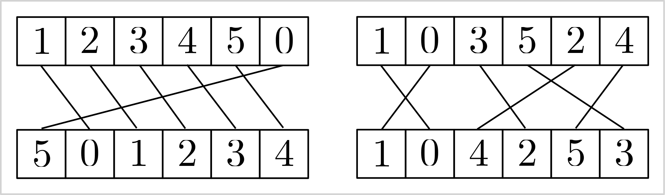 |
|---|
Visualizing the stable matching induced by the add_inverse constraint. |
Warning
I generally advise against using the add_element and add_inverse
constraints. While CP-SAT may have effective propagation techniques for them,
these constraints can appear unnatural and complex. It's often more
straightforward to model stable matching with binary variables add_exactly_one constraint for each vertex to ensure unique matches. If your
model needs to capture specific attributes or costs associated with
connections, binary variables are necessary. Relying solely on indices would
require additional logic for accurate representation. Additionally, use
non-binary variables only if the numerical value inherently carries semantic
meaning that cannot simply be re-indexed.