DWD (Distance Weighted Discrimination) is a linear classification algorithm, similar to an SVM. It considers the input data as some high-dimensional space and determines some hyperplane which bisects that space. Data on each side of the hyperplane is classified together.
Although this distance is actually a euclidean distance, since the space has such high dimension it is more useful to interpret it as a "confidence"; cases far from the separation are more strongly associated with the corresponding class. Using the distance as a new "severity" metric with which we can do further analysis.
The typical workflow for the module is:
- Define input dataset(s) and tuning parameter(s). ShapeVariationAnalyzer can be used to do this.
- Train a model and validate training statistics
- Apply the model to a testing dataset to generate detailed results
- Analyze these results or correlate them with additional metrics
All datasets used in SlicerDWD should use the same csv format as in ShapeVariationAnalyzer. Testing and Training datasets should have columns Filename and Group.
Additional numerical metrics may be used; the first column of these datasets must also be Filename. Note that Filename is used as a key to match metrics with testing samples.
The "Split Training and Testing Data" option allows to specify a single dataset, which is used for both training and testing. A configurable percentage of the training dataset will be removed and used for testing. This is a good way to validate the model can perform well on new data to avoid overfitting. If the option is disabled, then training and testing datasets must be provided separately. It is possible to use the same dataset for training as for testing in this way, although it is not recommended as overfitting cannot be detected.
DWD exposes one hyperparameter, C, the penalty for mis-classifications. It is possible to manually set this value, however this is not advised as it can easily lead to overfitting to the training data. The auto-generated value for C is typically a sufficiently balanced value to prevent overfitting.
Once a training dataset has been selected, click "Train Classifier" to build and fit a DWD classifier. Some statistics of the classifiers performance on the training data will be shown: overall accuracy, and precision and recall for each class. Ideally all of these values will be close to 100%; however it is important to also test the classifier on unseen data to avoid overfitting.
Once a testing dataset is selected, click "Test Classifier" to generate the same accuracy, precision, and recall statistics. These can be used for validating the model on unseen data.
Testing also generates a table, listing the predicted class and confidence (Distance) for each case in the testing set. These results can be saved to a file with the "Save Test Results" option, or viewed in the table widget within the module.
Once test results are generated, analysis may be performed over the results.
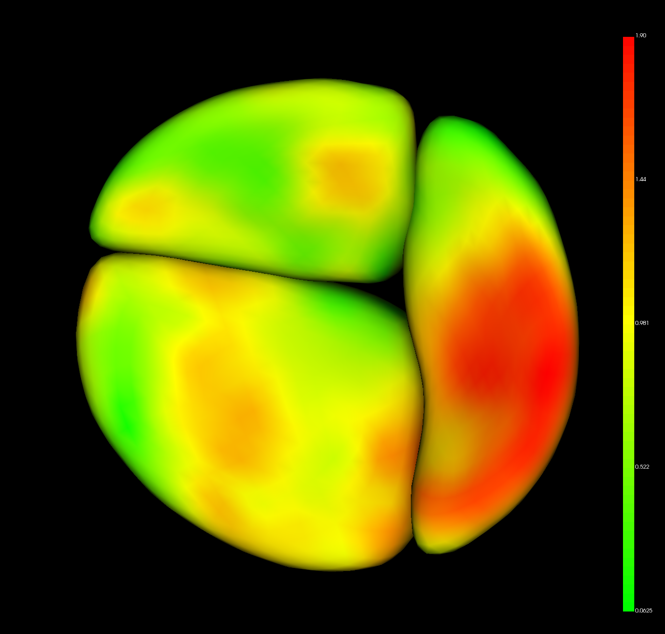
This operation averages the shape of all the testing data, and projects the resulting model to DWD separating plane. The result can be interpreted as a shape-wise "midpoint" between the two classes. The model is opened in ShapePopulationViewer.
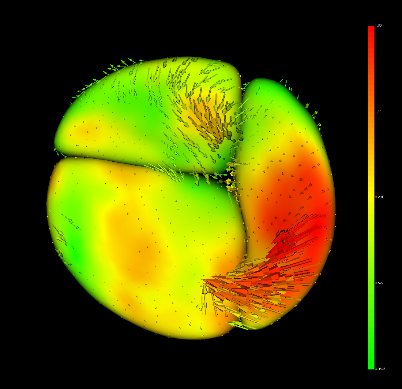
The resulting model also has the DWD direction stored as point data. In ShapePopulationViewer, find the "ColorMap and Vectors" group and choose the "Vectors" tab. Enable "Display Vectors" to visualize the DWD direction. If each point on the model were moved in the indicated direction, then DWD would classify it in the first Group. The result can be interpreted as a shape-wise "significance" which DWD is uses to classify data.
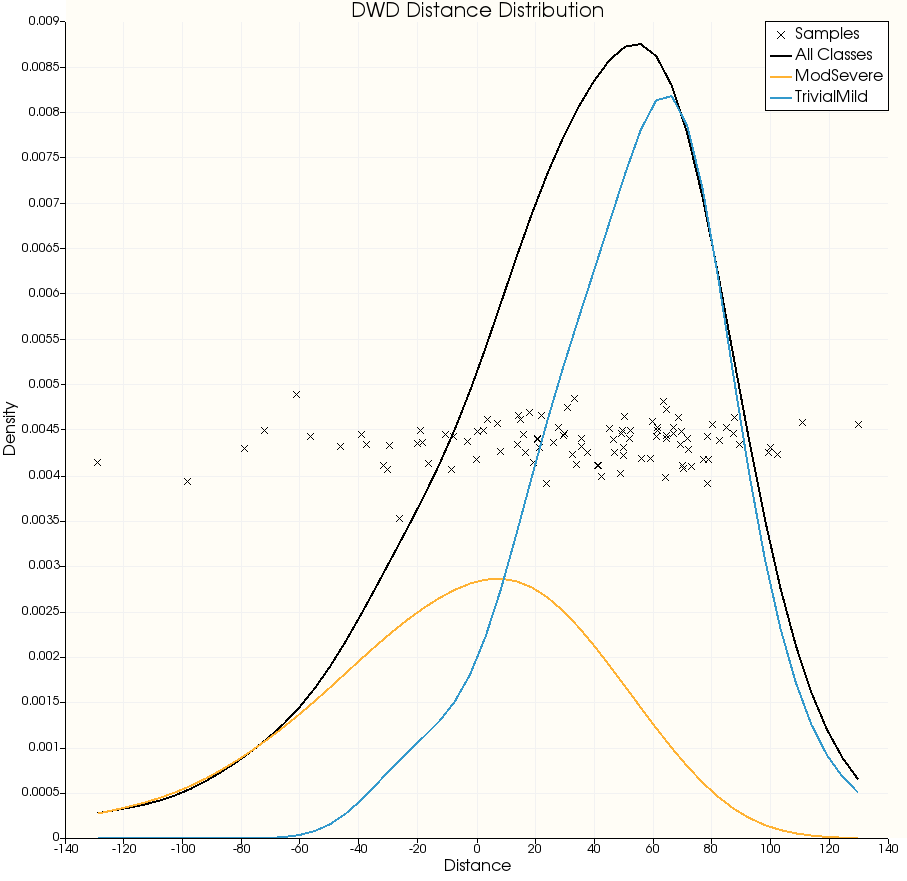
This operation visualizes the distribution of cases along the DWD separating direction; it is useful to be able to see how confident DWD is in its classification of certain samples, and how the cases of each class are distributed by that metric.
The KDE (Kernel Density Estimation) assigns a "density" to the distribution of samples; more samples will be located in regions where the KDE is high. This can be useful when there are many samples as it is easier to read than a collection of point markers.
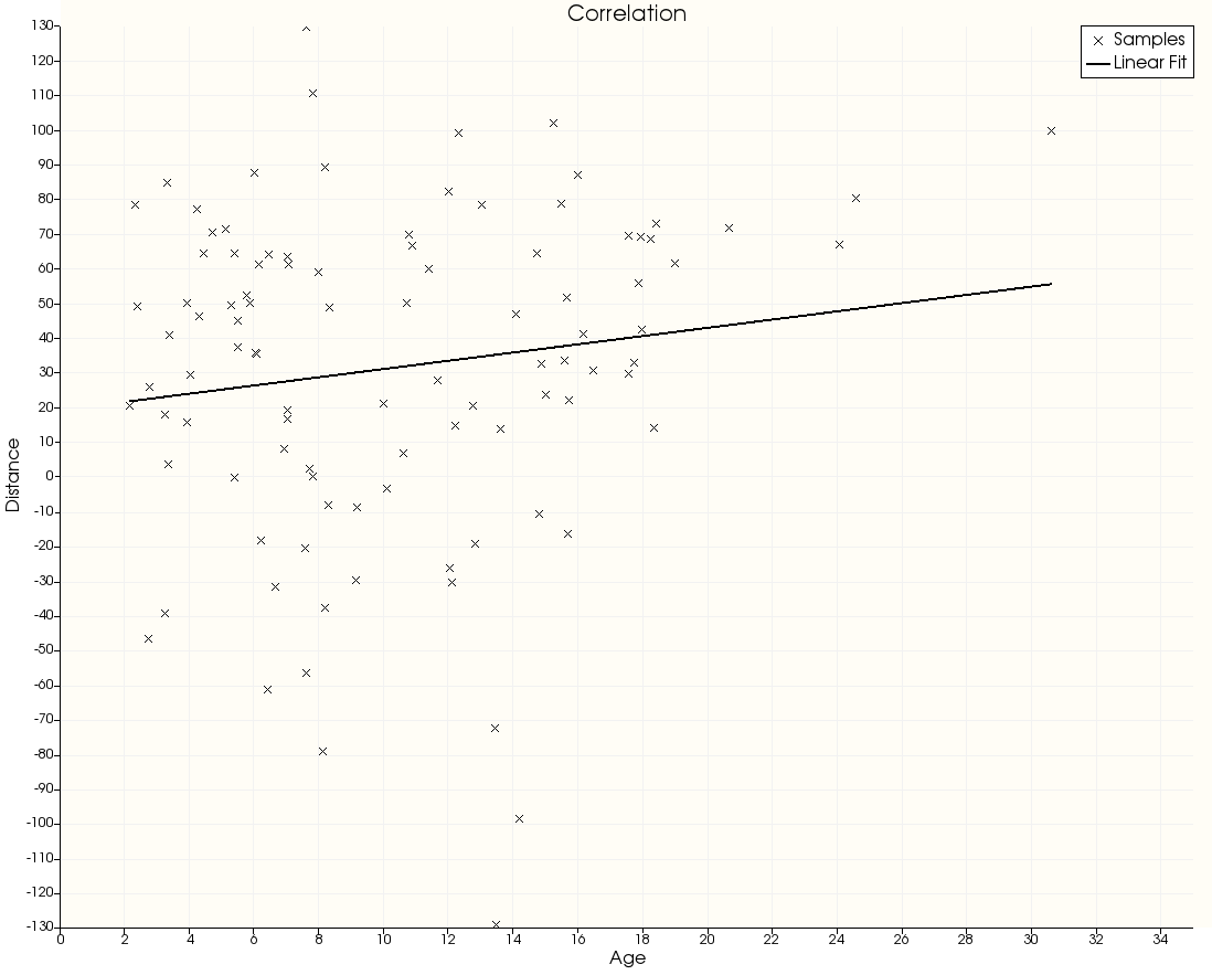
This operation correlates the distance with some other numerical metric. Use the drop-down to choose a column in the metrics dataset to plot the distance against that metric, along with a linear regression.