Point pattern analysis is a statistical technique used to analyze the patterns formed by points in a space, particularly clustering versus dispersion of observations. We can utilize the spatstat package in order to go through various functions which quantify clustering and dispersion throughout our dataset. This script outlines how you would conduct a spatial point pattern analysis!

0. Load in Packages

require(spatstat)
require(spatstat.data)
require(spdep)
require(sf)
require(here)

1. Prepare Data

# Load in Data
pts <- read.csv(here("data", "cactus.csv"))
boundary <- read.csv(here("data", "cactus_boundaries.csv"),header=T)

# Create a spatstat object  with our pts data
ppp.window <- owin(xrange=c(boundary$Xmin, boundary$Xmax),
                   yrange=c(boundary$Ymin, boundary$Ymax))
ppp <- ppp(pts$East, pts$North, window=ppp.window)

2. Plot raw data and density

par(mfrow = c(1,2), oma=c(0,0,0,1))
plot(ppp, main = "Points")
plot(density(ppp,1), main = "Density")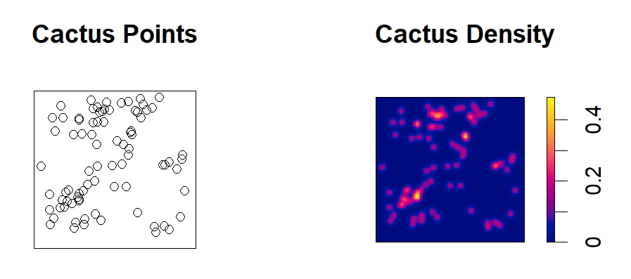

3. Take a look at the data's ppp summary

summary(ppp)

4. Ripleys K with various corrections

# K 1:1 expectation (no correction)
Knone <- Kest(ppp, correction="none")

# K with Isotropic edge correction
Kiso <- Kest(ppp, correction="isotropic")

# K with Translate (toroidal) edge correction
Ktrans <- Kest(ppp, correction="trans")

# Plot
ppp_plot("K", Knone, Kiso, Ktrans)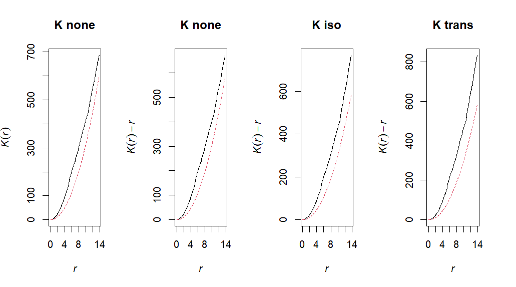

5. L with various corrections

# L 1:1 expectation (no correction)
Lnone <- Lest(ppp, correction="none")

# L with Isotropic edge correction
Liso <- Lest(ppp, correction="isotropic")

# L with Translate (toroidal) edge correction
Ltrans <- Lest(ppp, correction="trans")

# Plot
ppp_plot("L", Lnone, Liso, Ltrans)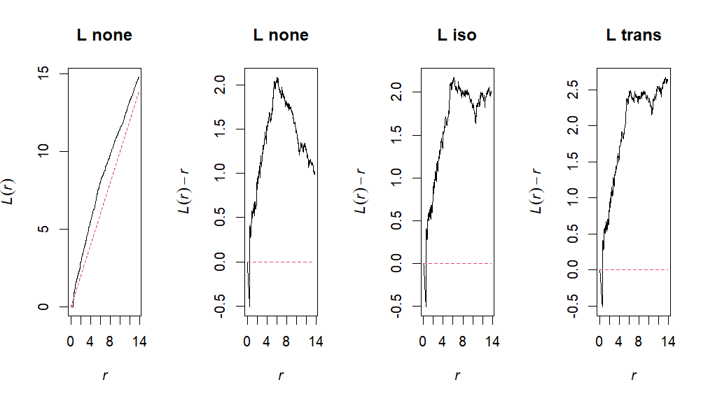

6. Pair correlation function, g, with various corrections

# g 1:1 expectation (no correction)
Pnone <- pcf(ppp, correction="none")

# g with Isotropic edge correction
Piso <- pcf(ppp, correction="isotropic")

# g with Translate (toroidal) edge correction
Ptrans <- pcf(ppp, correction="trans")

# Plot
par(mfrow = c(1,3))
plot(Pnone, main = "Pnone",legend=F, ylim=c(0,3))         
plot(Piso, main = "Piso", legend=F, ylim=c(0,3))
plot(Ptrans, main = "Ptrans", legend=F, ylim=c(0,3))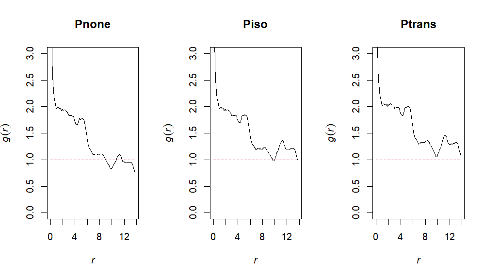

7. G Function with various corrections

# G 1:1 expectation (no correction)
Gnone <- Gest(ppp, correction="none")

# G with Reduced sample or border correction
Grs <- Gest(ppp, correction="rs")

# G with Best (determines best correction for dataset)
Gbest = Gest(ppp, correction="best")

# Plot!
par(mfrow = c(1,3))
plot(Gnone, main = "Gnone",legend=F)         
plot(Grs, main = "Grs", legend=F)
plot(Gbest, main = "Gbest", legend=F)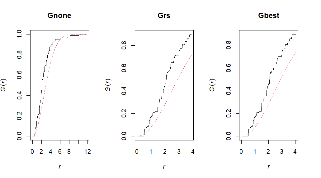

8. F Function with various corrections

# F 1:1 expectation (no correction)
Fnone <- Fest(ppp, correction="none")

# F with Reduced sample or border correction
Frs <- Fest(ppp, correction="rs")

# F with Best (determines best correction for dataset)
Fbest = Fest(ppp, correction="best")

# 9.4: Plot!
par(mfrow = c(1,3))
plot(Fnone, main = "Fnone",legend=F)         
plot(Frs, main = "Frs", legend=F)
plot(Fbest, main = "Fbest", legend=F)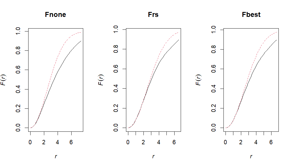

9. Point Pattern Process Envelopes

Create a Lest simulated envelope of global and pointwise confidence under CSR

# Create a global & pointwise (non-global) Envelope
Lcsr   <- envelope(ppp, Lest, nsim=99, rank=1, correction="trans", global=F)
Lcsr.g <- envelope(ppp, Lest, nsim=99, rank=1, correction="trans", global=T)

# Plot point-wise envelope
plot(Lcsr, . - r~r, shade=c("hi", "lo"), legend=F)

# Plot global envelope
plot(Lcsr.g, . - r~r, shade=c("hi", "lo"), legend=F)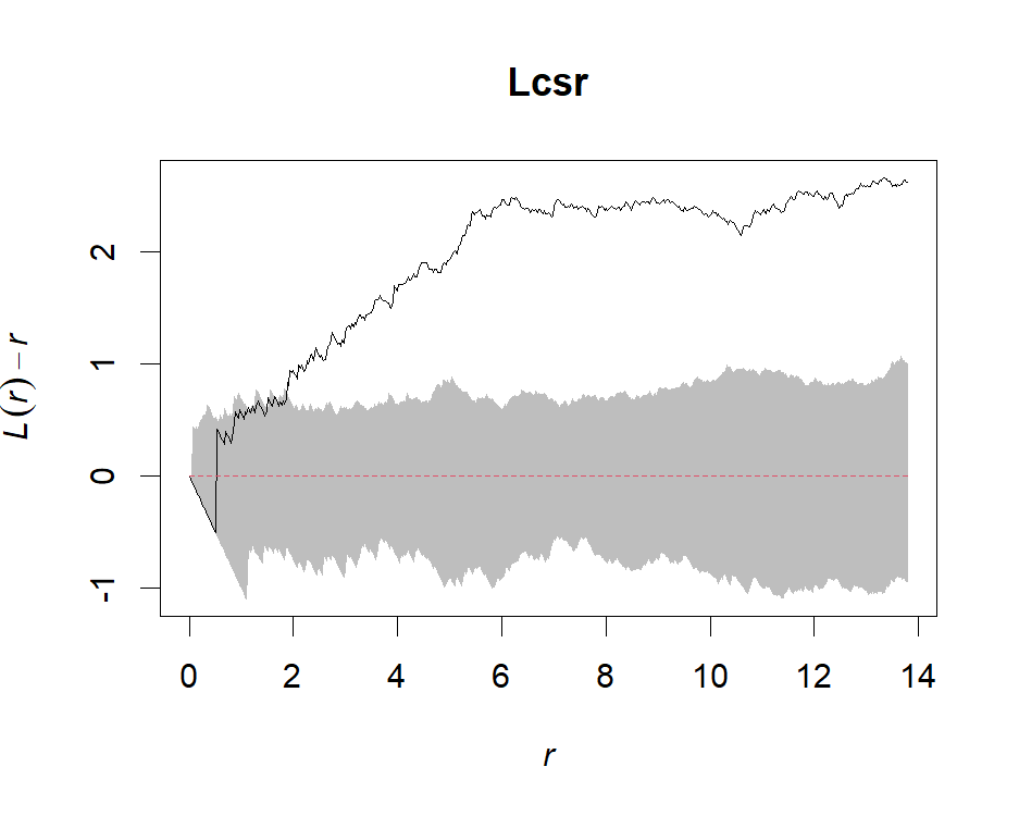

Create a pcf simulated envelope of pointwise confidence under CSR

# Create a fine envelope
Penv <- envelope(ppp,pcf, nsim=99, rank=1, stoyan=0.15, correction="trans", global=F)#stoyan = bandwidth; set to default

# Create a coarse envelope
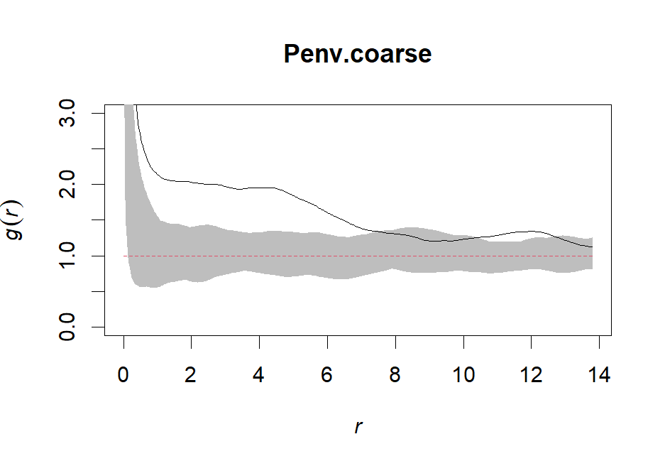
Penv.coarse <- envelope(ppp, pcf, nsim=99, rank=1, stoyan=0.3, correction="trans", global=F)

# Plot our fine envelope
plot(Penv, shade=c("hi", "lo"), legend=FALSE, ylim = c(0,3))

# Plot our coarse envelope
plot(Penv.coarse, shade=c("hi", "lo"), legend=F, ylim = c(0,3))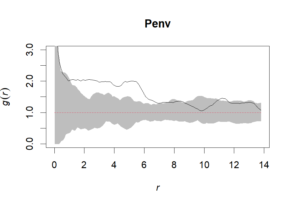

Create a Gest simulated envelope of pointwise confidence under CSR

# Create a pointwise Gest envelope
Genv <- envelope(ppp, Gest, nsim=99, rank=1, correction="rs", global=F)

# Create a nearest neighbor distance variable for our plot
nn.dist <- nndist(ppp)
max(nn.dist)

# Plot our trans G
plot(Gtrans, legend=F)

# Plot G with our pointwise envelope & nearest neighbor distances
plot(Genv, shade=c("hi", "lo"), legend=F)
plot(ecdf(nn.dist), add=T)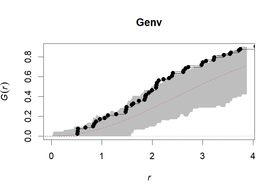

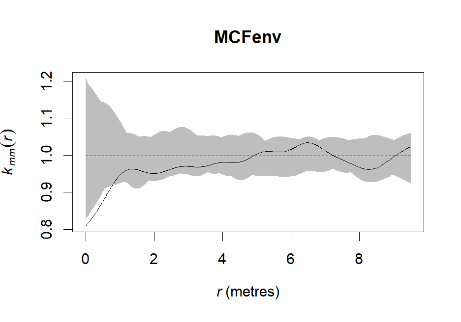
10. Mark-Correlation Analysis

# Load in our example dataset
data(spruces)

# Create an envelope for spruces
MCFenv <- envelope(spruces, markcorr, nsim=99, correction="iso", global=F)

# Plot envelope
plot(MCFenv,  shade=c("hi", "lo"), legend=F)