Combining Radial Basis Function Networks with Convolutional Neural Networks

Before the advent of Convolutional Neural Networks (CNNs), Radial Basis Function Neural Networks (RBFs) were popular in image recognition and computer vision tasks. However, RBFs’ lack of adaptability to modern architecture has prevented their integration with deep learning computer vision research.

Here in this article, we will try to combine these network architectures to develop something that gives us the best of both worlds!

Table of Contents:

1. What is a RBF?
2. Why combine it with a CNN?
3. Problems in combining
4. Tackling the Problems
5. Conclusion
6. References

What is an RBF?

RBFs are mathematically defined as a global approximation method of a mapping $F$ from a $d$ dimensional feature space to a $K$ dimensional label space $(F:~IR^d\rightarrow IR^K)$^[1]. In simpler words, it is a mixed unsupervised and supervised machine learning tool that categorizes multi-dimensional data into different classes.

The RBF architecture consists of an input layer, a hidden layer containing cluster centres $(c_j)$, and an output layer. The cluster centres are separately learned, generally by using the KNN algorithm.

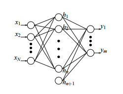
During the evaluation, also known as inference, distance is calculated between the input and the cluster centres, and an activation function is applied to the obtained distance. Mathematically:

$$ \begin{align} r^2 = ||x^\mu -c_j||^2_{R_j} = (x-c_j)^TR_j(x-c_j) \\ y_k = F_k(x) = \sum^C_{j=1}w_{jk}h(||x^\mu -c_j||^2_{R_j}) + w_{0k} \end{align} $$

Where $r$ represents the distance, $R_j$ is the positive definite covariance matrix (trainable distance), $T$ denotes the matrix transposition, $w_{jk}$ shows the weights of the output layers, $h$ is the activation function, and $w_{0k}$ are the biases. In these equations, $\mu$, $j$, and $k$ enumerate the number of samples, cluster centres, and classes, respectively. The output weights, cluster centres, and covariance matrix are the trainable part of the above equations.

The distance $r$ computed in equation $(1)$ is not only a measure of the proximity of an input point to a cluster centre but can also be used to compare different inputs and find similar and dissimilar samples in the input space.

Some of the commonly used activation functions when RBFs are deployed are as follows^[2]:

$$ \begin{align} h(r)&=r \\ h(r)&=e^{-\frac{r^2}{2\sigma^2}} \\ h(r)&=r^2\ln{r} \\ h(r)&=\frac{1}{1+r^2/\sigma^2} \end{align} $$

We can summarise the training of these networks in 3 steps^[3]:

• (a) Unsupervised Learning:

  This step aims to find cluster centres representative of the data. The k-means clustering algorithm is widely used for this purpose. k-means iteratively finds a set of cluster centres and minimizes the overall distance between cluster centres and members over the entire dataset. The target of the k-means algorithm can be written in the following form:

  $$ \begin{align} \text{Loss}{unsupervised} = \sum^K{j=1}\sum_{x^\mu \in v_j}||x^\mu -c_j||^2 \end{align} $$

  Where $x^\mu \in v_j$ denotes the members of the $j^{th}$ cluster shown by $v_j$.

• (b) Computing Weights:

  The output weights of an RBF network can be computed using a closed-form solution. The matrix of activation of the samples is defined from the training set $(H)$ as follows:

  $$ \begin{align} H = h(||x^\mu -c_j||^2_{R_j})_{\mu=1,...,M,~j=1,...,C} \end{align} $$

  Based on equation $(2)$, the matrix of output weights $(W)$, which estimates the matrix of labels $(Y)$, is computed by the following equation:

  $$ \begin{align} Y \approx MW \implies W \approx M^\dagger Y \end{align} $$

  Where $M^\dagger$ is the Moore-Penrose pseudo-inverse matrix of $H$ and is computed as:

  $$ \begin{align} H^\dagger = \lim_{\alpha\rightarrow0^+}(H^TH+\alpha I)^{-1}H^T \end{align} $$

• (c) End-to-End Optimization:

  After initializing the RBF weights and cluster centres with clustering algorithms such as k-means, optimizing the network end-to-end via backpropagation and gradient descent is possible.

Why combine it with a CNN?

In recent times, CNNs have become the go-to architecture for computer vision tasks thanks to their ability to produce their filters on their own. No manual Feature extraction! These models have also performed successfully in industry, only helping their growth.

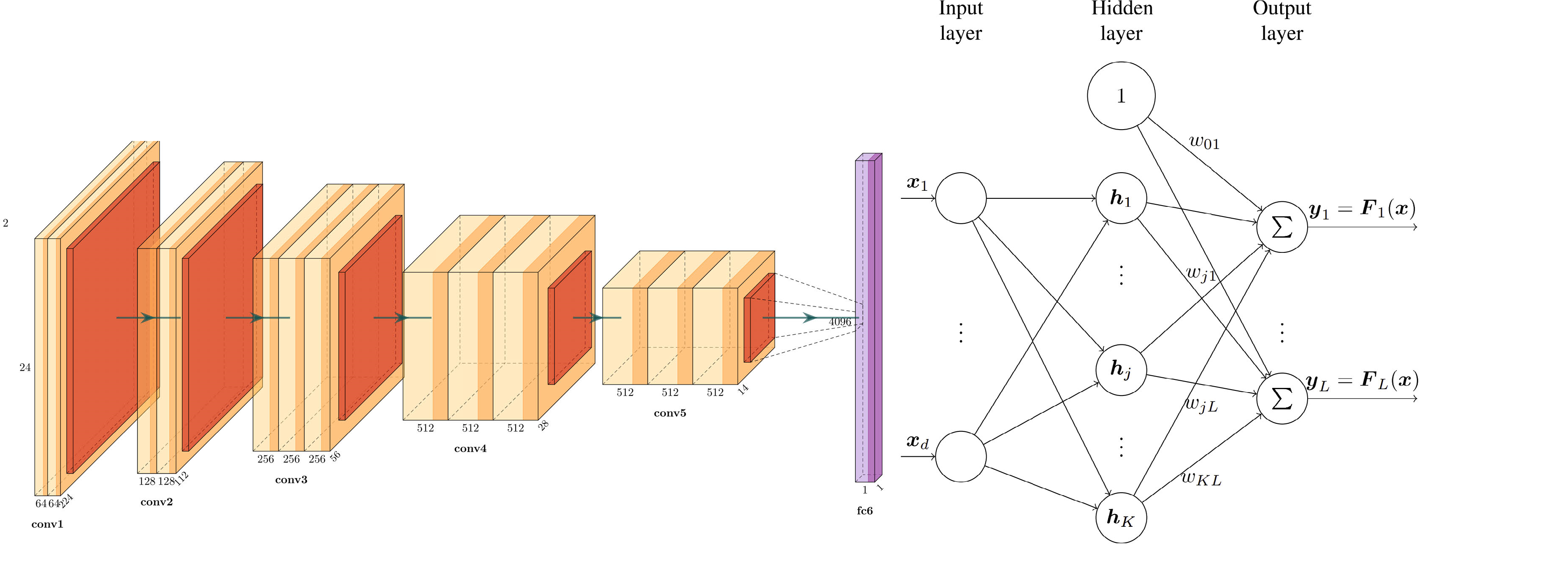
Despite all this, if there is something that CNNs lack, then it is the interpretability of the trained model. How exactly the model is classifying things sometimes is not very intuitive. This drawback can be tackled by adding an RBF-like model at the end of a CNN to enhance the interpretability while adding some non-linear complexity to the entire model.

Apart from adding interpretability to the model, the addition of the RBF would also provide us with a new distance metric $(r)$. This metric can be used as a similarity metric; similar is the distances of a pair of items to their cluster centre, similar they are. The metric can help us find similar/dissimilar items within a classified label.

To summarize:

• Enhancement in Interpritiblity
• Obtainment of a Similarity Metric
• Addition of non-linearity

are the fundamental motivation behind combining RBFs with CNNs.

Problems in combining

Although combining these models is advantageous, it is not as easy as just adding one at the end of another. There are many architectural limitations which prevent us from doing so. They are as follows:

• (a) Initialization: Training the RBFs from scratch with randomly initialized weights using gradient descent is relatively inefficient due to inappropriate initial cluster centres. The large initial distances in high dimensional spaces lead to small activation values, and the gradients attenuate considerably after the RBF hidden layer during backpropagation. Furthermore, computing the weights from equation $(9)$ is not feasible at the scale of computer vision problems such as ImageNet, which has over 14 million images and 1000 classes.

• (b) Dynamic Input Features:

  The input features of classical RBFs are fixed, but this assumption is not valid concerning CNNs. As the embeddings of CNNs develop during the training process, the cluster centres initialized by the k-means algorithm are no longer optimal after a few training epochs.

• (c) Activation:

  The non-linear computational graph drawn by computing the distance in equation $(1)$ and applying the activations in equations $(3)$-$(6)$ leads to inefficient gradient flow.

Tackling the Problems

The problems mentioned above can be solved in the following ways:

• (a) Initialization: To tackle the large initial distances, we can use the k-means algorithm to initialize the cluster centres before starting the training. We can randomly initialize the output layer and optimize it for the computational issues using gradient descent rather than the closed form solution.

• (b) Dynamic Input Features: The problem of changing input features can be tackled by adding an “unsupervised” part to the overall model’s loss function. This unsupervised part can be thought of as applying the KNN algorithm while training the model. The loss function mentioned in equation $(7)$ can be used for this purpose. Thus the final loss function of the model would look like this,

  $$ \begin{align} \text{Loss} = \text{Loss}{supervised} + \lambda \text{Loss}{unsupervised} \end{align} $$

  Where the classification loss $(\text{Loss}_{supervised})$ is any arbitrary loss function, for instance categorical cross entropy.

• (c) Activation: The problem of inefficient backpropagation can be solved using a new activation function. The quadratic activation proposed by Amirian^[4] can be used here. The proposed activation is:

  $$ \begin{align} h(r)=1-\frac{r^2}{\sigma^2} \end{align} $$

  Where $\sigma$ is the parameter that determines the width of the kernel. The activation kernel can be visually compared with standard kernels in the following image.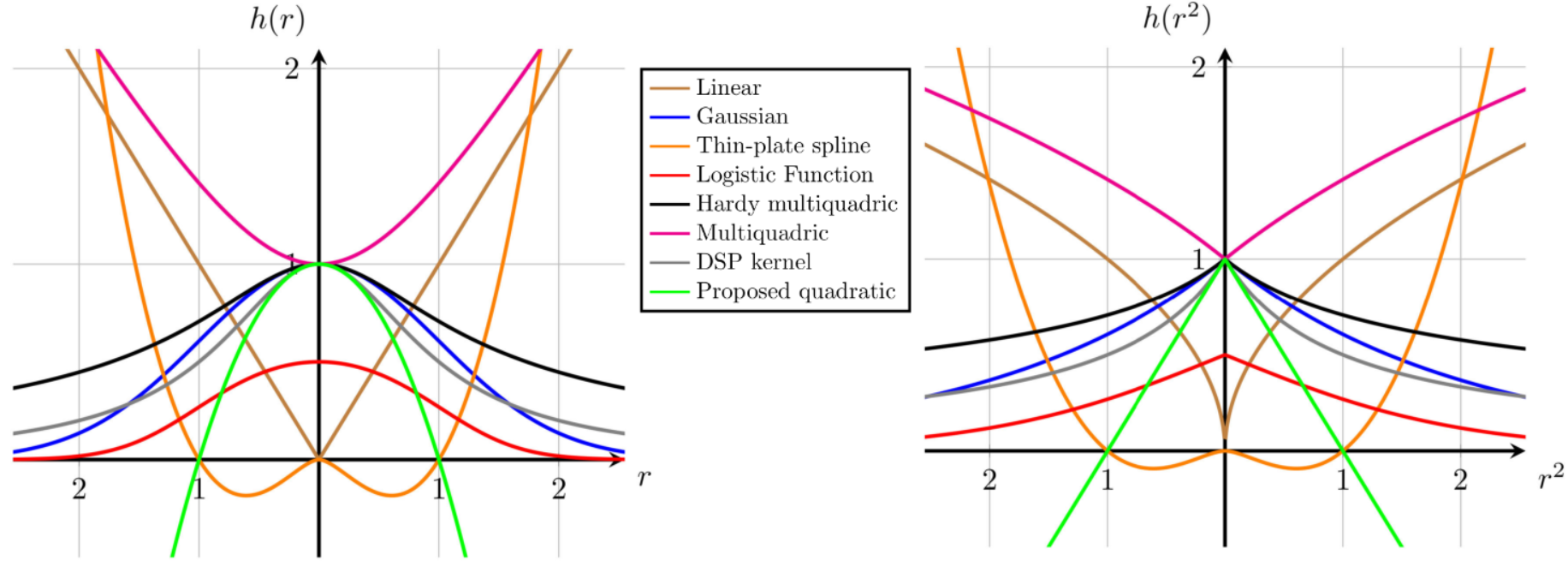

  

  The proposed quadratic kernel reduces the non-linearity of the CNN-RBF computational graph for backpropagation.

After making the above changes, the RBF is ready to be integrated with any CNN we want!

Conclusion

The combination model of an RBF and a CNN is quite powerful. Even if it does not improve the accuracy by much, the interpretability it gives is invaluable in understanding how a CNN is classifying the input. The similarity metric is also handy for finding something like “The most non-Pomerian Dog” or “The most Labrador-ish Dog”.

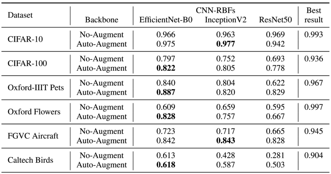
The above-described model was tested^[4] on various standard image classification datasets to get the following results.

References:

[1]: D. Broomhead and D. Lowe, “Multivariable functional interpolation and adaptive networks, complex systems,” Tech. Rep, vol. 2, 1988.

[2]: T. Poggio and F. Girosi, “Networks for approximation and learning,” Proc. IEEE Inst. Electr. Electron. Eng., vol. 78, no. 9, pp. 1481–1497, 1990.

[3]: F. Schwenker, H. A. Kestler, and G. Palm, “Three learning phases for radial-basis-function networks,” Neural Netw., vol. 14, no. 4–5, pp. 439–458, 2001.

[4]: M. Amirian and F. Schwenker, “Radial basis function networks for convolutional neural networks to learn similarity distance metric and improve interpretability,” IEEE Access, vol. 8, pp. 123087–123097, 2020.