jq-voronoi

Implementation of Fortune's algorithm to calculate Voronoi diagram on jq

Try it

Clone this repository. To run the following jq must be installed and availbale on PATH.

$ ./gensites | ./voronoi.sh | ./2svg --argjson box '[600, 600]' > /tmp/voronoi.svg

Check generated file /tmp/voronoi.svg.

Usage

Algorithm takes as input list of sites (points of two-dimentional plane) and returns as output a list of voronoi cells (polygons delimiting zone of influence of sites). Script voronoi/voronoi.jq (or wrapper voronoi.sh) takes as input array of points in cartesian coordinates.
Consider the following example:

as JSON:

[[0, 0], [100, 100], [20, 15], [60, 10], [90, 20], [45, 40], [25, 65], [65, 80]]

First two points are coordinates of respectively top-left & bottom-right corners of bounding box. The rest are coordinates of sites that must imperatively be within bounding box.
Script outputs an array of cells. Cell is an JSON array where the first element is a site, and the rest are counter-clockwise ordered points forming polygon of voronoi cell of this site.

[
  [
    /* Coordinates of site */
    [20, 15],
    
    /* Counter-clockwise ordered points forming polygon of voronoi cell of the site */
    [40.833333333333336, 19.166666666666668],
    [38.43749999999999, 0],
    [0, 0],
    [0, 42.25000000000001],
    [19.72222222222222, 40.27777777777778]
  ],
  ...   // other sites  
]

Visualization:

Render to SVG

Tool 2svg can render calculated voronoi diagram into SVG file.

Usage:

$ echo '[[0, 0], [100, 100], ... ]' | ./voronoi.sh | ./2svg --argjson box '[100, 100]' > output.svg

2svg takes a single JSON argument box, defining bounding box. box can have 2 or 4 elements.

Two elements (Example: [600, 600])
Box starts at [0, 0]

1. box width = 600
2. box height = 600

Four elements (Example: [50, 50, 150, 150])

1. top-left corner x = 50
2. top-left corner y = 50
3. bottom-right corner x = 150
4. bottom-right corner y = 150

Examples:

$ ./2svg --argjson box '[600, 600]'             # bounding box [0, 0] -> [600, 600]
$ ./2svg --argjson box '[50, 50, 150, 150]'     # bounding box [50, 50] -> [150, 150]

Voronoi diagram for [[0, 0], [100, 100], [20, 15], [60, 10], [90, 20], [45, 40], [25, 65], [65, 80]]:

Visualization sketch

Voronoi diagram can also be displayed by sketch.
To run visualization sketch Processing 3+ must be installed and processing-java executable must be on the PATH.
Redirect output of voronoi.sh (voronoi/voronoi.jq) to display. Script accepts two or four parameters, defining bounding box.
If user supplies two arguments, they are respectively width & height of the bounding box starting at [0, 0].
If user provides four arguments, the two first arguments are x & y coordinates of top-left corner, and last two are x & y coordinates of bottom-right corner of bounding box.

Examples:

$ display 600 600             # bounding box [0, 0] -> [600, 600]
$ display 50 50 150 150       # bounding box [50, 50] -> [150, 150]

To test visualisation:

$ ./gensites | ./voronoi.sh | ./display 600 600

Voronoi on sphere

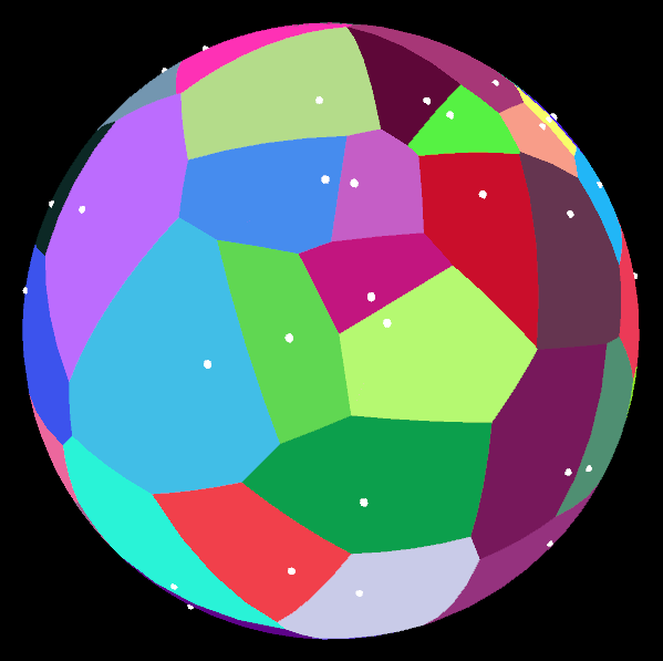
Computation of Voronoi diagram on spherical surface is based on paper "Voronoi diagrams on the sphere" by Hyeon-Suk Na, Chung-Nim Lee & Otfried Cheong. Spherical Voronoi diagram is obtained in time O(n log n) from two planar Voronoi diagrams and a little bit of glueing.

In order to compute Voronoi on sphere we must supply sites expressed in spherical coordinates on unit sphere [φ, θ], where

    0 ≤ φ ≤ 2π (azimuth)
    0 ≤ θ ≤ π  (zenith)

Coordinate [0, 0] defines a north pole.

Example:

$ echo '[[1, 1.5], [1, 1], [1, 2.2]]' | ./voronoi.sh --sphere

Visualisation is done by Processing sketch:

$ ./gensites-sphere | ./voronoi.sh -s | ./display-sphere