
- gather some colleagues and make a team of maximum 3 people
- choose a topic that you would like to research; propose your own or check the project list
- make sure your topic does not overlap with other topics that are in progress and that have been chosen by your colleagues
- email sergiu to announce your team, your proposal and to discuss how to approach it
- after you obtain the approval, mark it as being in progress on the kanban list, and start working on it
- prepare the project, a presentation, and a report using this template
- place everything in a digital storage space somewhere: a git repo, a drive, some file on a server etc.; don’t send large files by email, send only URLs
- current deadline for completing projects: January 20
- Three Thousand Years of Algorithmic Rituals: The Emergence of AI from the Computation of Space, Matteo Pasquinelli
- Excerpt:
The term “algorithm” comes from the Latinization of the name of the Persian scholar al-Khwarizmi. His tract On the Calculation with Hindu Numerals, written in Baghdad in the ninth century, is responsible for introducing Hindu numerals to the West, along with the corresponding new techniques for calculating them, namely algorithms. In fact, the medieval Latin word “algorismus” referred to the procedures and shortcuts for carrying out the four fundamental mathematical operations—addition, subtraction, multiplication, and division—with Hindu numerals. Later, the term “algorithm” would metaphorically denote any step-by-step logical procedure and become the core of computing logic. In general, we can distinguish three stages in the history of the algorithm: in ancient times, the algorithm can be recognized in procedures and codified rituals to achieve a specific goal and transmit rules; in the Middle Ages, the algorithm was the name of a procedure to help mathematical operations; in modern times, the algorithm qua logical procedure becomes fully mechanized and automated by machines and then digital computers.
Looking at ancient practices such as the Agnicayana ritual and the Hindu rules for calculation, we can sketch a basic definition of “algorithm” that is compatible with modern computer science:
- an algorithm is an abstract diagram that emerges from the repetition of a process, an organization of time, space, labor, and operations: it is not a rule that is invented from above but emerges from below;
- an algorithm is the division of this process into finite steps in order to perform and control it efficiently;
- an algorithm is a solution to a problem, an invention that bootstraps beyond the constrains of the situation: any algorithm is a trick;
- most importantly, an algorithm is an economic process, as it must employ the least amount of resources in terms of space, time, and energy, adapting to the limits of the situation.
Today, amidst the expanding capacities of AI, there is a tendency to perceive algorithms as an application or imposition of abstract mathematical ideas upon concrete data. On the contrary, the genealogy of the algorithm shows that its form has emerged from material practices, from a mundane division of space, time, labor, and social relations.
- Language, Cohesion and Form (Studies in Natural Language Processing), Margaret Masterman, Yorick Wilks
- The Perceptron, Frank Rosenblatt
- Calculating Space, Konrad Zuse
- Algorithmic Theories of Everything, Jürgen Schmidhuber
- Theory of Self-Reproducing Automata, John von Neumann
- Inference in an Authorship Problem, Frederick Mosteller and David L. Wallace
Excerpts:
As statisticians, our interest in this controversy is largely methodological. Problems of discrimination are widespread, and we wished a case study that would give us an opportunity to compare the more usual methods of discrimination with an approach via Bayes’ theorem.
[...]
The classical approach to discrimination problems, flowing from Fisher’s "linear discriminant function" and from the Neyman-Pearson fundamental lemma, is well exposited by Rao 10, Chapter 8. Important recent writings on Bayesian statistics include the books by Jeffries 6, by Raiffa and Schlaifer 9, and by Savage 11
[...]
Let us look in Table 2.1 at frequency distributions for rates of the high-frequency words by, from, and to in 48 Hamilton and 50 Madison papers (some exterior to The Federalist®). [Table 2.1. contains frequency distribution of rates per thousand words for the 48 Hamilton and 50 Madison papers.] High rates for by usually favor Madison, low favor Hamilton; for to the reverse holds. Low rates for from tell little, but high rates favor Madison. In Table 2.2, we see that rates for the word war vary considerably for both authors. The meaning of war automatically suggests that the rate of use of this word depends on the topic under discussion. In discussions of the armed forces the rate is expected to be high; in a discussion of voting, low. We call words with such variable rates "contextual" and we regard them as dangerous for discrimination.
[...]
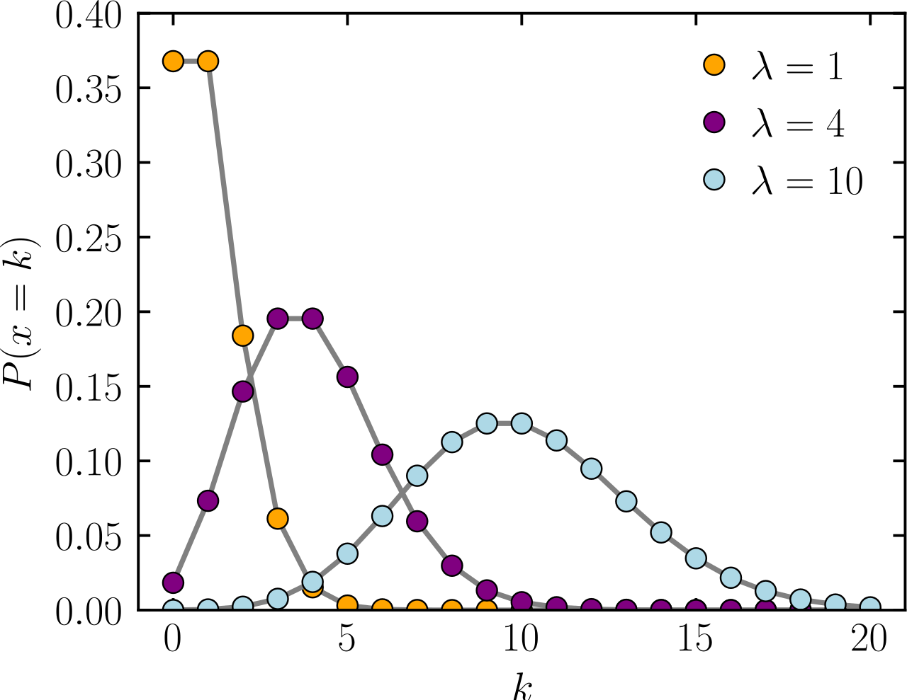
Nearly all words have low rates per thousand words; thus the occurrence of any one word at one spot in a text is a rare event. In many statistical problems distributions of rare events are governed by the Poisson law, which gives the probability of a count of
Modern books designate the counts by
[...]
To find out how well the Poisson fits the distribution of Hamilton and Madison word counts, we broke up a collection of Federalist papers into 247 blocks of approximately 200 words, and tabulated the frequency distribution of counts for each of many different words we give distributions for Hamilton in Table 2.4.
[observed values contain the number of blocks where the word has been observed 0 times, 1 time, etc. Poisson values are computed using the function above
The distributions for an, any, and upon are fitted rather well by the Poisson, but even a motherly eye1 sees disparities for may and his.
|
|
0 | 1 | 2 | 3 | 4 | 5 | 6 | 7 or more |
|---|---|---|---|---|---|---|---|---|
| an observed | 77 | 89 | 46 | 21 | 9 | 4 | 1 | |
| an Poisson | 71.6 | 88.6 | 54.9 | 22.7 | 7.0 | 1.7 | 4 | 1 |
| any observed | 125 | 88 | 26 | 7 | 0 | 1 | ||
| any Poisson | 126.3 | 84.6 | 28.5 | 6.4 | 1.1 | 2 |
[...]
Let
Let
The conditional probability that Hypothesis 1 is true given observation
Both computational and intuitive advantages accrue if we use odds instead of probabilities. [...]
The logarithmic form of Bayes’ theorem can be obtained by taking the logarithm:
The initial odds [priors]
Suppose Hamilton’s and Madison’s use of the word also are well represented by Poisson distributions with parameters
So, assuming Poisson distribution, for a single word with frequency
then the log-likelyhood ratio between hypotheses
Based on the Naive assumption that words appear independently in a text, and the authors decision to set the priors as equally probable (
where
- Understanding of Multinomial Naive Bayes for Text Classification, Jurafsky and Martin
- Chapter 8 - Discrimination Problems, Radhakrishna Rao
- Bayesian statistics, Jeffries
- Bayesian statistics, Raiffa and Schlaifer
- Bayesian statistics, Savage
This is part of a wider philosophical regarding language and cognition. We shall only lift up the dust from these debates and point to the most lowdly-heard opinions.

A înţelege o propoziţie înseamnă a înţelege un limbaj. A înţelege un limbaj înseamnă a stăpîni o tehnică. Cum explic eu cuiva semnificaţia cuvintelor "regulat", "uniform", "acelaşi"? Unuia care, să zicem, nu vorbeşte decât franceză, îi voi explica aceste cuvinte prin cuvintele franţuzeşti corespunzătoare. Dar cine nu posedă încă aceste noţiuni, pe acela îl voi învăţa să folosească cuvintele prin exemple şi prin exerciţiu. Şi cînd fac asta, nu-i comunic mai puţin decît ştiu eu însumi. Wittgenstein, Cercetări Filozofice
“For a large class of cases of the employment of the word ‘meaning’—though not for all—this word can be explained in this way: the meaning of a word is its use in the language” (PI 43). This basic statement is what underlies the change of perspective most typical of the later phase of Wittgenstein’s thought: a change from a conception of meaning as representation to a view which looks to use as the crux of the investigation. Traditional theories of meaning in the history of philosophy were intent on pointing to something exterior to the proposition which endows it with sense. This ‘something’ could generally be located either in an objective space, or inside the mind as mental representation. As early as 1933 (The Blue Book) Wittgenstein took pains to challenge these conceptions, arriving at the insight that “if we had to name anything which is the life of the sign, we should have to say that it was its use” (BB 4).

QUESTION: What role does cognition play in the acquisition and development of language? Do linguistic factors influence general cognitive development?
CHOMSKY: I would like to re-phrase the first question and ask what role other aspects of cognition play in the acquisition of language since, as put, it is not a question I can answer. I would want to regard language as one aspect of cognition and its development as one aspect of the development of cognition. It seems to me that what we can say in general is this:
There are a number of cognitive systems which seem to have quite distinct and specific properties. These systems provide the basis for certain cognitive capacities — for simplicity of exposition, I will ignore the distinction and speak a bit misleadingly about cognitive capacities. The language faculty is one of these cognitive systems. There are others. For example, our capacity to organize visual space, or to deal with abstract properties of the number system, or to comprehend and appreciate certain kinds of musical creation, or our ability to make sense of the social structures in which we play a role, which undoubtedly reflects conceptual structures that have developed in the mind, and any number of other mental capacities. As far as I can see, to the extent that we understand anything about these capacities, they appear to have quite specific and unique properties. That is, I don’t see any obvious relationship between, for example, the basic properties of the structure of language as represented in the mind on the one hand and the properties of our capacity, say, to recognize faces or understand some situation in which we play a role, or appreciate music and so on. These seem to be quite different and unique in their characteristics. Furthermore, every one of these mental capacities appears to be highly articulated as well as specifically structured. Now it’s perfectly reasonable to ask how the development of one of these various systems relates to the development of others. Similarly, in the study of, say, the physical growth of the body, it makes perfect sense to ask how the development of one system relates to the development of others. Let’s say, how the development of the circulatory system relates to the development of the visual system.
But in the study of the physical body, nobody would raise a question analogous to the one you posed in quite this form. That is, we we would not ask what role physical organs and their function play in the development of the visual system. Undoubtedly, there are relations between, say, the visual and circulatory systems, but the way we approach the problem of growth and development in the physical body is rather different. That is, one asks — quite properly — what are the specific properties and characteristics of the various systems that emerge — how do these various organs or systems interact with one another, what is the biological basis — the genetic coding, ultimately — that determines the specific pattern of growth, function and interaction of these highly articulated systems: for instance, the circulatory system, the visual system, the liver, and so on. And that seems to provide a reasonable analogy, as a point of departure at least, for the study of cognitive development and cognitive structure, including the growth of the language faculty as a special case.

URL here short version on wikipedia, trilingual PDF here
A game on a stadium where people act according to mechanical and logical instructions to produce a translation from Portuguese.
"Outcries and laughter filled the hall for quite a while. Zarubin laughed with us. Then he shook his notebook in the air and, when the hall was silent again, he read slowly: “Os maiores resultados sao produzidos роr – pequenos mas continues esforcos”.
This is a sentence in Portuguese. I don’t think you can guess what it means. However, it was you who yesterday made a perfect Russian translation. Here it is: “The greatest goals are achieved through minor but continuous ekkedt.”
“Remember that part of Turing’s article in which he said that to find out whether machines are able to think, you have to become a machine. Experts in cybernetics believe that the only way to prove that machines can think is to turn yourself into a machine and examine your thinking process.
Hence, yesterday we spent four hours operating like a machine. Not a fictional one, but a serial, domestic machine named Ural. If we had more people, we could have worked as Strela, Large Electronic Computing Machine, or any other computing machine. I decided to try Ural and used you, my dear young friends, as elements to build it at the stadium. I prepared a program to translate Portuguese texts, did the encoding procedure, and placed it into the “memory unit” – the Georgian delegation. I gave the grammatical rules to our Ukrainian colleagues, and the Russian team was responsible for the dictionary.
Our machine handled the mission flawlessly, as the translation of the foreign sentence into Russian required absolutely no thinking. You definitely understand that such a living machine could solve any mathematical or logical problem just like state-of-the-art electronic computing machines. However, that would require much more time. And now let us try to answer one of the most critical questions of cybernetics: Can machines think?”
“No!” everyone roared.
“I object!” yelled our “cybernetics nut,” Anton Golovin. “During the game we acted like individual switches or neurons. And nobody ever said that every single neuron has its own thoughts. A thought is the joint product of numerous neurons!”
“Okay,” the Professor agreed. “Then we have to assume that during the game the air was stuffed with some ‘machine superthoughts’ unknown to and inconceivable by the machine’s thinking elements! Something like Hegel’s noûs, right?”
Golovin stopped short and sat down.
“If you, being structural elements of some logical pattern, had no idea of what you were doing, then can we really argue about the ‘thoughts’ of electronic devices made of different parts which are deemed incapable of any thinking even by the most fervent followers of the electronic-brain concept? You know all these parts: radio tubes, semiconductors, magnetic matrixes, etc. I think our game gave us the right answer to the question ‘Can machines think?’ We’ve proven that even the most perfect simulation of machine thinking is not the thinking process itself, which is a higher form of motion of living matter. And this is where I can declare the Congress adjourned.”

- image from Pygmalion displacement paper
- The Thinking Machine documentary from the '60s where the is moderator smoking a pipe nonchalantly.
I ask you to watch who are the people doing the actual research. Worth noting minute 10:31 where somebody is being tested2. To understand more about the context, see the recent Pygmalion displacement paper by Lelia A. Erscoi, Annelies Kleinherenbrink, and Olivia Guest. Short excerpts below:
First, we examine the fictional fascination with AI, or minimally AI-like entities, e.g. automata, which are created with the explicit purpose to displace women by recreating artificially their typical social role (examples shown on the left and in pink in Figure 2).
In the section titled Fictional Timeline, we trace the ways in which the misogyny expressed in the original telling of the Pygmalion myth has been echoed and transmuted over time, culminating in films like “Ex Machina” and “Her” in the 21st century.
We follow up this analysis of Pygmalion-inspired fiction with a discussion of the work of Alan Turing3, in the section titled Interlude: Can Women Think?. Even though the Turing test is now widely understood to involve a machine being mistaken for a human — any human — the original test re volved around a computer being mistaken specifically for a woman (Genova, 1994).
We therefore argue that Turing’s thought experiment can be seen as a case of Pygmalion displacement (i.e. the humanization of AI through the dehumanization of women). As such, it serves as a noteworthy bridge between fictional and actual attempts to replace women with machines. After this ‘interlude’, we develop our Pygmalion lens (Table 1), which is described in detail in the section titled The Pygmalion lens: real myths or mythical realities?.
In a further twist of dramatic irony, as we already alluded to above, the original Turing test is another instance of Pygmalion displacement. Turing introduces his original formulation of the test by means of “a game which we call the ‘imitation game’.
It is played with three people, a man (A), a woman (B), and an interrogator (C) who may be of either sex. [...] The object of the game for the third player (B) is to help the interrogator. The best strategy for her is probably to give truthful answers. She can add such things as ‘I am the woman, don’t listen to him!’ to her answers, but it will avail nothing as the man can make similar remarks.” (pp. 433–434) Turing (1950) then asks “‘What will happen when a machine takes the part of A [the man] in this game?’ Will the interrogator decide wrongly as often when the game is played like this as he does when the game is played between a man and a woman? These questions replace our original, Can machines think? (p. 434)
This description of the second test leaves some room for interpretation (Brahnam et al., 2011). The majority of interpretations suggest that Turing intends this second game as a test of human-likeness, in general, not of gender specifically (cf. Guest & Martin, 2023, wherein related but separate problems with adopting the test uncritically in the scientific study of brain and cognition are discussed).
[...]
Turing invites us to accept that to convince the interrogator of their humanity, human-likeness, or both, machine and woman could answer questions that probe things like their ability to play masculinised games like chess (viz. Keith, 1994), but not patriarchal female-coded characteristics. “We do not wish to penalise the machine for its inability to shine in beauty competitions” (Turing, 1950, p. 435).
In an alternative reading, however, the judge is still tasked with figuring out which player is a woman, and the computer is programmed specifically to prove it is a woman (Genova, 1994; Kind, 2022). “Turing actually said that the method of the test was by imitating gender[, thus] the function to be performed [by the machine] is the imitation of a female person” (Keith, 1994, p. 334).
If this was indeed Turing’s intention, the computer imitates a man imitating (and outsmarting) a woman, and thus still emulates masculine thinking (Brahnam et al., 2011). In both understandings of the test, the machine is arguably not required to be exactly like women (defined in terms of stereotypes), in fact it has to surpass them by reproducing masculine thinking skills (again, stereotypically defined).

The neuroscience of perception has recently been revolutionized with an integrative modeling approach in which computation, brain function, and behavior are linked across many datasets and many computational models. By revealing trends across models, this approach yields novel insights into cognitive and neural mechanisms in the target domain. We here present a systematic study taking this approach to higher-level cognition: human language processing, our species’ signature cognitive skill. We find that the most powerful “transformer” models predict nearly 100% of explainable variance in neural responses to sentences and generalize across different datasets and imaging modalities (functional MRI and electrocorticography). Models’ neural fits (“brain score”) and fits to behavioral responses are both strongly correlated with model accuracy on the next-word prediction task (but not other language tasks). Model architecture appears to substantially contribute to neural fit. These results provide computationally explicit evidence that predictive processing fundamentally shapes the language comprehension mechanisms in the human brain.
To evaluate model candidates of mechanisms, we use previously published human recordings: fMRI activations to short passages (Pereira et al., 2018), ECoG recordings to single words in diverse sentences (Fedorenko et al., 2016), fMRI to story fragments (Blank et al. 2014). More specifically, we present the same stimuli to models that were presented to humans and “record” model activations. We then compute a correlation score of how well the model recordings can predict human recordings with a regression fit on a subset of the stimuli. Since we also want to figure out how close model predictions are to the internal reliability of the data, we extrapolate a ceiling of how well an “infinite number of subjects” could predict individual subjects in the data. Scores are normalized by this estimated ceiling.
So how well do models actually predict our recordings? We tested 43 diverse language models, incl. embedding, recurrent, and transformer models. Specific models (GPT2-xl) predict some of the data near perfectly, and consistently across datasets. Embeddings like GloVe do not. The scores of models are further predicted by the task performance of models to predict the next word on the WikiText-2 language modeling dataset (evaluated as perplexity, lower is better) – but NOT by task performance on any of the GLUE benchmarks.
- from the original 2021 paper
- Highly recommended presentation by Ev Fedorenko
- Automating Gender: Postmodern Feminism in the Age of the Intelligent Machine, Judith Halberstam
- Pygmalion Displacement: When Humanising AI Dehumanises Women, Erscoi, L., Kleinherenbrink, A., & Guest, O.
- Language Is a Poor Heuristic For Intelligence, Karawynn Long
- Reclaiming AI as a theoretical tool for cognitive science, van Rooij, I., Guest, O., Adolfi, F. G., de Haan, R., Kolokolova, A., & Rich, P.
- The neural architecture of language: Integrative modeling converges on predictive processing, Schrimpf, M., Blank, I., Tuckute, G., Kauf, C., Hosseini, E., Kanwisher, N., Tenenbaum, J., Fedorenko, E
- Other Papers from the Brain and Language Lab
- On Chomsky and the Two Cultures of Statistical Learning, debate with P. Norvig
- Does a language model trained on “A is B” generalize to “B is A”?, Lukas Berglund, Meg Tong, Max Kaufmann, Mikita Balesni, Asa Cooper Stickland, Tomasz Korbak, Owain Evans
- Unthought: the power of the cognitive nonconscious, Katherine Hayles
- The Future Looms: Weaving Women and Cybernetics, Sadie Plant
You will often hear or read that probabilities for words are estimated using a maximum likelihood estimator by counting the number of occurences to the total. But what is "maximum likelihood"?
Remember the following two basic rules of probabilities:
- conditional probability of two events
$A$ and$B$ not independent: $$ \text{1. } P(A,B) = P(A)*P(A|B) \ = P(B,A) = P(B)*P(B|A) $$ - marginal probability as the sum of all partitions $$ \text{2. } P(B) = \sum_{A_i}P(B, A_i) = \sum_{A_i}P(B|A_i)P(A_i) $$
From rule 1. we get Bayes' theorem: $$ P(A|B) = \frac{P(A)P(B|A)}{P(B)} \ posterior = \frac{prior * likelihood}{marginal} $$ which is equivalent to saying "we update our beliefes after the evidence is considered".
Hopefully it is more clear now, that if we talk about maximum likelihood estimation, it might have something to do likelihood term
Let's start with the simplest example: we have a binary coin that returns 0, 1. We don't know at this point if the coin has been rigged and we want to use data (observed trials) to define a set of beliefes. Which one is more likely 0 or 1? Are they really equally probable?
Common sense would say each coin has the same probability, e.g., the probability of seeing
By seeing something, here we mean that we have some observations or some data
\begin{align} f(k; \theta) = P(k;\theta) = p_{\theta}(k)&={\begin{cases}\theta&{\text{if }}k=1,\1-\theta&{\text{if }}k=0.\end{cases}} \ &= \theta^k(1-\theta)^{(1-k)} \end{align}
We could also model the data as a Binomial distribution, which describes the success of
\begin{equation} {\displaystyle f(c,N,\theta)=P(c;N,\theta)=p_{\theta, N}(c)={\binom {N}{c}}\theta^{c}(1-\theta)^{N-c}} \end{equation}
We use different notations in PMF to make it clear that different textbooks refer to the same thing.
We know the Bernouli distribution is parameterized by
- what are the most likely parameters
$\theta$ of the Bernouli probability distribution$P_{\theta}(\cdots)$ that explain the data$D = {x_1, x_2, ..., x_N}$ ? let's note this as$\hat{\theta}$ - one might encounter the parameters writted with a column
$P(\cdots ; \theta)$ or defined as a separate function ${\mathcal {L}}(\theta \mid \cdots) = {\mathcal {L}}(\theta) = {\mathcal {L}}{N}(\theta )={\mathcal {L}}{N}(\theta ; \cdots )=f_{N}(\cdots ;\theta );$ - we use
$\cdots$ do signify any notation for data, here we will used$D$ , but$\mathbf{y}$ is also often encountered; sometimes the data is ommited completely${\mathcal {L}}(\theta)$
Bayesian statistics allows treating these parameters as coming from a distribution while frequentist statistics does not allow distributions of unobserved variables (such as parameters). Causal models (see Bayesian statistics course here) start by modelling a generating process of the data. For a brief comparison between Bayesian and frequentist statistics, see this blog post. Maximum likelihood estimation is inherently a frequentist approach. Keep in mind that this is not the only approach to estimate the parameters from the data.
The formal textbook definition of the likelihood function in frequentist statistics is written in multiple ways, depending on the textbook:
$$
{\mathcal {L}}(\theta \mid x) = P(X=x; \theta) =p_{\theta }(x) =P_{\theta }(X=x)
$$
representing the probability of observing the outcome
By the Maximum Likelihood Estimation, we mean the parameter
$$
\hat{\theta}{\text{MLE}} = \operatorname*{argmax}{\theta} P_{\theta}(D)
$$
For independent and identically distributed random variables iid, such as our dataset
For our coin, these are individual Bernoullis and we have a parameter
$$ p_{\theta}(1) = \theta ,\ p_{\theta}(0) = 1-\theta $$ therefore
$$ \begin{align} \hat{\theta} &= \operatorname*{argmax}{\theta} {\mathcal {L}}(D | \theta) \ \hat{\theta} &= \operatorname*{argmax}{\theta} \prod_{i=1}^{N} p_{\theta}(x_i) \ &= \operatorname*{argmax}{\theta} \prod{i=1}^{N} \theta^{x_i}(1-\theta)^{(1-x_i)} \ \end{align} $$
To maximize the function we can:
- use log values (log-likelihood
$l(\theta) = log{\mathcal{L}}(\theta)$ to aid our computation (we can do this because the log is monotonic and the likelihood is positive) - take the derivative and equate with zero to find points of extreme
- check the second derivative is negative to make sure it's not a point of minimum
the sums above can be denoted as two constants defined by counts:
then if we equate with zero: $$ \frac{\partial\mathcal{l}(\theta)}{\partial \theta} = \frac{\partial c\log\theta + (N - c)\log(1-\theta)}{\partial \theta} = 0 $$ and we get $$ c\frac{1}{\theta} - (N-c)\frac{1}{1-\theta} = 0 \ c(1-\theta) = (N-c)\theta \ $$ therefore $$ \hat{\theta} = \frac{c}{N} = \frac{\sum_{i=1}^{N}x_i}{N} $$
which is equivalent to saying that the maximum likelihood estimator is the relative frequency of an event: the number of counts of an event divided by the total number.
Long story short, MLE estimation is a means to derive the parameters that best describe a set of observations by doing a derivative over parameters using the probability mass/density function across a dataset.
In the above example with
A first solution would be to introduce some smoothing constants (or hallucinations) in the estimator, suppose we add
This can be arbitrary? How many new samples should we add after all?
To tackle this problem, we can break the frequentist assumption that parameters are not observable events. Thus, we apply Bayesian statistics and assume that
But we can still use Bayes' Theorem and find the best parameter
We have the following terminology:
-
$P(\theta \mid D)$ posterior probabilities after observing the data -
$P(\theta)$ priors -
$P(D\mid \theta)$ likelihood, can be defined as the PMF or PDF -
$P(D)$ the marginals which sometimes are denoted by$Z$ , are usually untractable, and treated as a normalizing factor since they do not impact$\operatorname*{argmax}_{\theta}$ . The marginals may also be encountered as the sum of all partitions or an integral.
The maximum a posteriori is about finding the best parameters that explain our data by modelling the posterior probabilities: $$ \begin{align} \hat{\theta}{\text{MAP}} &= \operatorname*{argmax}{\theta} P(\theta \mid D) \ &= \operatorname*{argmax}{\theta} P(D\mid \theta) P(\theta) \ &= \operatorname*{argmax}{\theta} \log P(D\mid \theta) + \log P(\theta) \end{align} $$
For the Binomial distribution, we were looking at a distribution to give us the probability of
Remember the Binomial distribution which is defined by the rate of success of
$$
Bin(c | \theta, N) = \begin{pmatrix} N \ c \end{pmatrix} \theta^c(1-\theta)^{d}
$$
where
$$
{\displaystyle \begin{pmatrix} N \ c \end{pmatrix} = \frac{N!}{c!(N-c)!} = \frac{(d+c)!}{c!d!} = \begin{pmatrix} d+c \ c \end{pmatrix}}
$$
represents combinations of N taken c.
The binomial distribution is a function that depends on
Since
The prior with the same functional form as the Binomial is called the Beta distribution given by:
$$
Beta(\theta | \alpha, \beta) = B(\alpha,\beta) * \theta^{(\alpha-1)} * (1-\theta)^{(\beta-1)}
$$
where
The $\Gamma$ function is the extension of the factorial function:
Unlike the Binomial (where we modelled the probability of successes
If we set
Now that we have a conjugate to model the parameter
$$
\begin{align}
P(\theta \mid D) &=
C(\alpha,\beta,c,d) * \theta^c(1-\theta)^{d} * \theta^{(\alpha-1)} * (1-\theta)^{(\beta-1)} \
&= C(\alpha,b,c,d) * \theta^{(c + \alpha-1)} * (1-\theta)^{(d+ \beta-1)} \
&\propto \theta^{(c + \alpha - 1)} * (1-\theta)^{(d + \beta - 1)} \
\end{align}
$$
where
It is clear now that using the conjugate form is advantageous for the posterior has the same functional dependency on
Getting back to our example of 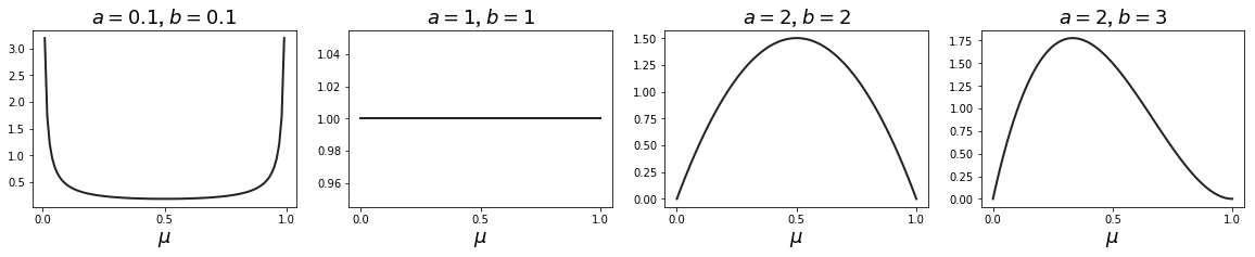
Furthermore, the posterior distribution can act as the prior if we subsequently observe additional data. To see this, we can imagine taking observations one at a time and after each observation updating the current posterior distribution by multiplying by the likelihood function for the new observation and then normalizing to obtain the new, revised posterior distribution. At each stage, the posterior is a Beta distribution with some total number of (prior and actual) observed
values for
Derive the MLE estimator for the parameters of a Gaussian distribution.
- Statistical Rethinking, consider starting with Chapter 2
- Maximum Likelihood course notes
- Comparison of MLE and MAP
- The Gamma Function, 1964, Emil Artin
- The Epic Story of Maximum Likelihood, Stephen M. Stiegler
- Conjugacy in Bayesian Inference, Gregory Gundersen
- First Links in the Markov Chain, Brian Hayes
- Entropia Limbii, 1963, Solomon Marcus & Sorin Stati
- A Mathematical Theory of Communication, 1948, Claude Shannon
- Prediction and Entropy of Printed English, 1951, Claude Shannon
- Easy-to-follow blog post on information theory
- Cybernetic Revolutionaries , Eden Medina
- Interview with Nils Gilman
Footnotes
-
even a motherly eye? worth noting a random sexist remark in an academic paper of the '60s ↩
-
ask youreself who is being tested and what game is being used. The river crossing problem is rooted in a history of sexism, racism, and colonialism. What were the missionaries doing there anyways? ↩
-
Alan Turing has been infamously persecuted for being LGBTQ+; also Wittgenstein was allegedly queer and strongly mysoginistic ↩